Gaussian process

From Wikipedia, the free encyclopedia

https://en.wikipedia.org/wiki/Gaussian_process 

In probability theory and statistics, a Gaussian process is a stochastic process (a collection of random variables indexed by time or space), such that every finite collection of those random variables has a multivariate normal distribution, i.e. every finite linear combination of them is normally distributed. The distribution of a Gaussian process is the joint distribution of all those (infinitely many) random variables, and as such, it is a distribution over functions with a continuous domain, e.g. time or space.

The concept of Gaussian processes is named after Carl Friedrich Gauss because it is based on the notion of the Gaussian distribution (normal distribution). Gaussian processes can be seen as an infinite-dimensional generalization of multivariate normal distributions.

Gaussian processes are useful in statistical modelling, benefiting from properties inherited from the normal distribution. For example, if a random process is modelled as a Gaussian process, the distributions of various derived quantities can be obtained explicitly. Such quantities include the average value of the process over a range of times and the error in estimating the average using sample values at a small set of times. While exact models often scale poorly as the amount of data increases, multiple approximation methods have been developed which often retain good accuracy while drastically reducing computation time.

Definition

A time continuous stochastic process ${\displaystyle \left\{X_t;t\in T\right\}}$ is Gaussian if and only if for every finite set of indices ${\displaystyle t_1,\dots ,t_k}$ in the index set ${\displaystyle T}$

$${\displaystyle {\mathbf{X}}_{t_1,\dots ,t_k}=(X_{t_1},\dots ,X_{t_k})}$$

is a multivariate Gaussian random variable. That is the same as saying every linear combination of ${\displaystyle (X_{t_1},\dots ,X_{t_k})}$ has a univariate normal (or Gaussian) distribution.

Using characteristic functions of random variables, the Gaussian property can be formulated as follows: ${\displaystyle \left\{X_t;t\in T\right\}}$ is Gaussian if and only if, for every finite set of indices ${\displaystyle t_1,\dots ,t_k}$, there are real-valued ${\displaystyle {\sigma }_{\ell j}}$, ${\displaystyle {\mu }_{\ell }}$ with ${\displaystyle {\sigma }_{jj}>0}$ such that the following equality holds for all ${\displaystyle s_1,s_2,\dots ,s_k\in \mathbb{R}}$

$${\displaystyle \mathrm{E}\left(\exp \left(i\sum _{\ell =1}^k{s}_{\ell }{\mathbf{X}}_{t_{\ell }}\right)\right)=\exp \left(-\frac{1}{2}\sum _{\ell ,j}{\sigma }_{\ell j}{s}_{\ell }{s}_j+i\sum _{\ell }{\mu }_{\ell }{s}_{\ell }\right),}$$

where ${\displaystyle i}$ denotes the imaginary unit such that ${\displaystyle i^2=-1}$.

The numbers ${\displaystyle {\sigma }_{\ell j}}$ and ${\displaystyle {\mu }_{\ell }}$ can be shown to be the covariances and means of the variables in the process.

Variance

The variance of a Gaussian process is finite at any time ${\displaystyle t}$, formally

$${\displaystyle \mathrm{var}[X(t)]=\mathrm{E}\left[{\left|X(t)-\mathrm{E}[X(t)]\right|}^2\right]<\mathrm{\infty }\text{for all }t\in T.}$$

Stationarity

For general stochastic processes strict-sense stationarity implies wide-sense stationarity but not every wide-sense stationary stochastic process is strict-sense stationary. However, for a Gaussian stochastic process the two concepts are equivalent.

A Gaussian stochastic process is strict-sense stationary if, and only if, it is wide-sense stationary.

Example

There is an explicit representation for stationary Gaussian processes. A simple example of this representation is

$${\displaystyle X_t=\cos (at){\xi }_1+\sin (at){\xi }_2}$$

where ${\displaystyle {\xi }_1}$ and ${\displaystyle {\xi }_2}$ are independent random variables with the standard normal distribution.

Covariance functions

Main article: Covariance function

Further information: Variogram

A key fact of Gaussian processes is that they can be completely defined by their second-order statistics. Thus, if a Gaussian process is assumed to have mean zero, defining the covariance function completely defines the process' behaviour. Importantly the non-negative definiteness of this function enables its spectral decomposition using the Karhunen–Loève expansion. Basic aspects that can be defined through the covariance function are the process' stationarity, isotropy, smoothness and periodicity.

Stationarity refers to the process' behaviour regarding the separation of any two points ${\displaystyle x}$ and ${\displaystyle x^{\prime }}$. If the process is stationary, the covariance function depends only on ${\displaystyle x-x^{\prime }}$. For example, the Ornstein–Uhlenbeck process is stationary.

If the process depends only on ${\displaystyle |x-x^{\prime }|}$, the Euclidean distance (not the direction) between ${\displaystyle x}$ and ${\displaystyle x^{\prime }}$, then the process is considered isotropic. A process that is concurrently stationary and isotropic is considered to be homogeneous; in practice these properties reflect the differences (or rather the lack of them) in the behaviour of the process given the location of the observer.

Ultimately Gaussian processes translate as taking priors on functions and the smoothness of these priors can be induced by the covariance function. If we expect that for "near-by" input points ${\displaystyle x}$ and ${\displaystyle x^{\prime }}$ their corresponding output points ${\displaystyle y}$ and ${\displaystyle y^{\prime }}$ to be "near-by" also, then the assumption of continuity is present. If we wish to allow for significant displacement then we might choose a rougher covariance function. Extreme examples of the behaviour is the Ornstein–Uhlenbeck covariance function and the squared exponential where the former is never differentiable and the latter infinitely differentiable.

Periodicity refers to inducing periodic patterns within the behaviour of the process. Formally, this is achieved by mapping the input ${\displaystyle x}$ to a two dimensional vector ${\displaystyle u(x)=\left(\cos (x),\sin (x)\right)}$.

Usual covariance functions

The effect of choosing different kernels on the prior function distribution of the Gaussian process. Left is a squared exponential kernel. Middle is Brownian. Right is quadratic.

There are a number of common covariance functions:

• Constant : ${\displaystyle K_{\mathrm{C}}(x,x^{\prime })=C}$
• Linear: ${\displaystyle K_{\mathrm{L}}(x,x^{\prime })=x^{\mathsf{T}}{x}^{\prime }}$
• white Gaussian noise: ${\displaystyle K_{\mathrm{GN}}(x,x^{\prime })={\sigma }^2{\delta }_{x,x^{\prime }}}$
• Squared exponential: ${\displaystyle K_{\mathrm{SE}}(x,x^{\prime })=\exp \left(-\frac{|d{|}^2}{2{\ell }^2}\right)}$
• Ornstein–Uhlenbeck: ${\displaystyle K_{\mathrm{OU}}(x,x^{\prime })=\exp \left(-\frac{|d|}{\ell }\right)}$
• Matérn: ${\displaystyle K_{\mathrm{Matern}}(x,x^{\prime })=\frac{2^{1-\nu }}{\mathrm{\Gamma }(\nu )}{\left(\frac{\sqrt{2\nu }|d|}{\ell }\right)}^{\nu }{K}_{\nu }\left(\frac{\sqrt{2\nu }|d|}{\ell }\right)}$
• Periodic: ${\displaystyle K_{\mathrm{P}}(x,x^{\prime })=\exp \left(-\frac{2{\sin }^2\left(\frac{d}{2}\right)}{{\ell }^2}\right)}$
• Rational quadratic: ${\displaystyle K_{\mathrm{RQ}}(x,x^{\prime })={\left(1+|d{|}^2\right)}^{-\alpha },\alpha \ge 0}$

Here ${\displaystyle d=x-x^{\prime }}$. The parameter ${\displaystyle \ell }$ is the characteristic length-scale of the process (practically, "how close" two points ${\displaystyle x}$ and ${\displaystyle x^{\prime }}$ have to be to influence each other significantly), ${\displaystyle \delta }$ is the Kronecker delta and ${\displaystyle \sigma }$ the standard deviation of the noise fluctuations. Moreover, ${\displaystyle K_{\nu }}$ is the modified Bessel function of order ${\displaystyle \nu }$ and ${\displaystyle \mathrm{\Gamma }(\nu )}$ is the gamma function evaluated at ${\displaystyle \nu }$. Importantly, a complicated covariance function can be defined as a linear combination of other simpler covariance functions in order to incorporate different insights about the data-set at hand.

The inferential results are dependent on the values of the hyperparameters ${\displaystyle \theta }$ (e.g. ${\displaystyle \ell }$ and ${\displaystyle \sigma }$) defining the model's behaviour. A popular choice for ${\displaystyle \theta }$ is to provide maximum a posteriori (MAP) estimates of it with some chosen prior. If the prior is very near uniform, this is the same as maximizing the marginal likelihood of the process; the marginalization being done over the observed process values ${\displaystyle y}$. This approach is also known as maximum likelihood II, evidence maximization, or empirical Bayes.

Continuity

For a Gaussian process, continuity in probability is equivalent to mean-square continuity, and continuity with probability one is equivalent to sample continuity. The latter implies, but is not implied by, continuity in probability. Continuity in probability holds if and only if the mean and autocovariance are continuous functions. In contrast, sample continuity was challenging even for stationary Gaussian processes (as probably noted first by Andrey Kolmogorov), and more challenging for more general processes. As usual, by a sample continuous process one means a process that admits a sample continuous modification. 

Stationary case

For a stationary Gaussian process ${\displaystyle X=(X_t{)}_{t\in \mathbb{R}},}$ some conditions on its spectrum are sufficient for sample continuity, but fail to be necessary. A necessary and sufficient condition, sometimes called Dudley–Fernique theorem, involves the function ${\displaystyle \sigma }$ defined by

$${\displaystyle \sigma (h)=\sqrt{\mathbb{E}(X(t+h)-X(t){)}^2}}$$

(the right-hand side does not depend on ${\displaystyle t}$ due to stationarity). Continuity of ${\displaystyle X}$ in probability is equivalent to continuity of ${\displaystyle \sigma }$ at ${\displaystyle 0.}$ When convergence of ${\displaystyle \sigma (h)}$ to ${\displaystyle 0}$ (as ${\displaystyle h\to 0}$) is too slow, sample continuity of ${\displaystyle X}$ may fail. Convergence of the following integrals matters:

$${\displaystyle I(\sigma )={\int }_0^1\frac{\sigma (h)}{h\sqrt{\log (1/h)}}dh={\int }_0^{\mathrm{\infty }}2\sigma (e^{-x^2})dx,}$$

these two integrals being equal according to integration by substitution $h=e^{-x^2},$ $x=\sqrt{\log (1/h)}.$ The first integrand need not be bounded as ${\displaystyle h\to 0+,}$ thus the integral may converge (${\displaystyle I(\sigma )<\mathrm{\infty }}$) or diverge (${\displaystyle I(\sigma )=\mathrm{\infty }}$). Taking for example $\sigma (e^{-x^2})=\frac{1}{x^a}$ for large ${\displaystyle x,}$ that is, $\sigma (h)=(\log (1/h){)}^{-a/2}$ for small ${\displaystyle h,}$ one obtains ${\displaystyle I(\sigma )<\mathrm{\infty }}$ when ${\displaystyle a>1,}$ and ${\displaystyle I(\sigma )=\mathrm{\infty }}$ when ${\displaystyle 0<a\le 1.}$ In these two cases the function ${\displaystyle \sigma }$ is increasing on ${\displaystyle [0,\mathrm{\infty }),}$ but generally it is not. Moreover, the condition

(*)   there exists ${\displaystyle \epsilon >0}$ such that ${\displaystyle \sigma }$ is monotone on ${\displaystyle [0,\epsilon ]}$

does not follow from continuity of ${\displaystyle \sigma }$ and the evident relations ${\displaystyle \sigma (h)\ge 0}$ (for all ${\displaystyle h}$) and ${\displaystyle \sigma (0)=0.}$

Theorem 1 — Let ${\displaystyle \sigma }$ be continuous and satisfy (*). Then the condition ${\displaystyle I(\sigma )<\mathrm{\infty }}$ is necessary and sufficient for sample continuity of ${\displaystyle X.}$

Some history. Sufficiency was announced by Xavier Fernique in 1964, but the first proof was published by Richard M. Dudley in 1967. Necessity was proved by Michael B. Marcus and Lawrence Shepp in 1970.

There exist sample continuous processes ${\displaystyle X}$ such that ${\displaystyle I(\sigma )=\mathrm{\infty };}$ they violate condition (*). An example found by Marcus and Shepp  is a random lacunary Fourier series

$${\displaystyle X_t=\sum _{n=1}^{\mathrm{\infty }}{c}_n({\xi }_n\cos {\lambda }_{n}t+{\eta }_n\sin {\lambda }_{n}t),}$$

where ${\displaystyle {\xi }_1,{\eta }_1,{\xi }_2,{\eta }_2,\dots }$ are independent random variables with standard normal distribution; frequencies ${\displaystyle 0<{\lambda }_1<{\lambda }_2<\dots }$ are a fast growing sequence; and coefficients ${\displaystyle c_n>0}$ satisfy $\sum _n{c}_n<\mathrm{\infty }.$ The latter relation implies $\mathbb{E}\sum _n{c}_n(|{\xi }_n|+|{\eta }_n|)=\sum _n{c}_n\mathbb{E}(|{\xi }_n|+|{\eta }_n|)=\text{const}\cdot \sum _n{c}_n<\mathrm{\infty },$ whence $\sum _n{c}_n(|{\xi }_n|+|{\eta }_n|)<\mathrm{\infty }$ almost surely, which ensures uniform convergence of the Fourier series almost surely, and sample continuity of ${\displaystyle X.}$

Autocorrelation of a random lacunary Fourier series

Its autocovariation function

$${\displaystyle \mathbb{E}{X}_t{X}_{t+h}=\sum _{n=1}^{\mathrm{\infty }}{c}_n^2\cos {\lambda }_{n}h}$$

is nowhere monotone (see the picture), as well as the corresponding function ${\displaystyle \sigma ,}$

$${\displaystyle \sigma (h)=\sqrt{2\mathbb{E}{X}_t{X}_t-2\mathbb{E}{X}_t{X}_{t+h}}=2\sqrt{\sum _{n=1}^{\mathrm{\infty }}{c}_n^2{\sin }^2\frac{{\lambda }_{n}h}{2}}.}$$

Brownian motion as the integral of Gaussian processes

A Wiener process (also known as Brownian motion) is the integral of a white noise generalized Gaussian process. It is not stationary, but it has stationary increments.

The Ornstein–Uhlenbeck process is a stationary Gaussian process.

The Brownian bridge is (like the Ornstein–Uhlenbeck process) an example of a Gaussian process whose increments are not independent.

The fractional Brownian motion is a Gaussian process whose covariance function is a generalisation of that of the Wiener process.

Driscoll's zero-one law

Driscoll's zero-one law is a result characterizing the sample functions generated by a Gaussian process.

Let ${\displaystyle f}$ be a mean-zero Gaussian process ${\displaystyle \left\{X_t;t\in T\right\}}$ with non-negative definite covariance function ${\displaystyle K}$. Let ${\displaystyle \mathcal{H}(R)}$ be a Reproducing kernel Hilbert space with positive definite kernel ${\displaystyle R}$.

Then

$${\displaystyle \underset{n\to \mathrm{\infty }}{lim}\mathrm{tr}[K_n{R}_n^{-1}]<\mathrm{\infty },}$$

where ${\displaystyle K_n}$ and ${\displaystyle R_n}$ are the covariance matrices of all possible pairs of ${\displaystyle n}$ points, implies

$${\displaystyle Pr[f\in \mathcal{H}(R)]=1.}$$

Moreover,

$${\displaystyle \underset{n\to \mathrm{\infty }}{lim}\mathrm{tr}[K_n{R}_n^{-1}]=\mathrm{\infty }}$$

implies 

$${\displaystyle Pr[f\in \mathcal{H}(R)]=0.}$$

This has significant implications when ${\displaystyle K=R}$, as

$${\displaystyle \underset{n\to \mathrm{\infty }}{lim}\mathrm{tr}[R_n{R}_n^{-1}]=\underset{n\to \mathrm{\infty }}{lim}\mathrm{tr}[I]=\underset{n\to \mathrm{\infty }}{lim}n=\mathrm{\infty }.}$$

As such, almost all sample paths of a mean-zero Gaussian process with positive definite kernel ${\displaystyle K}$ will lie outside of the Hilbert space ${\displaystyle \mathcal{H}(K)}$.

Linearly constrained Gaussian processes

For many applications of interest some pre-existing knowledge about the system at hand is already given. Consider e.g. the case where the output of the Gaussian process corresponds to a magnetic field; here, the real magnetic field is bound by Maxwell's equations and a way to incorporate this constraint into the Gaussian process formalism would be desirable as this would likely improve the accuracy of the algorithm.

A method on how to incorporate linear constraints into Gaussian processes already exists:

Consider the (vector valued) output function ${\displaystyle f(x)}$ which is known to obey the linear constraint (i.e. ${\displaystyle {\mathcal{F}}_X}$ is a linear operator)

$${\displaystyle {\mathcal{F}}_X(f(x))=0.}$$

Then the constraint ${\displaystyle {\mathcal{F}}_X}$ can be fulfilled by choosing ${\displaystyle f(x)={\mathcal{G}}_X(g(x))}$, where ${\displaystyle g(x)\sim \mathcal{G}\mathcal{P}({\mu }_g,K_g)}$ is modelled as a Gaussian process, and finding ${\displaystyle {\mathcal{G}}_X}$ such that

$${\displaystyle {\mathcal{F}}_X({\mathcal{G}}_X(g))=0\mathrm{\forall }g.}$$

Given ${\displaystyle {\mathcal{G}}_X}$ and using the fact that Gaussian processes are closed under linear transformations, the Gaussian process for ${\displaystyle f}$ obeying constraint ${\displaystyle {\mathcal{F}}_X}$ becomes

$${\displaystyle f(x)={\mathcal{G}}_{X}g\sim \mathcal{G}\mathcal{P}({\mathcal{G}}_X{\mu }_g,{\mathcal{G}}_X{K}_g{\mathcal{G}}_{X^{\prime }}^{\mathsf{T}}).}$$

Hence, linear constraints can be encoded into the mean and covariance function of a Gaussian process.

Applications

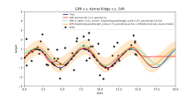
An example of Gaussian Process Regression (prediction) compared with other regression models.

A Gaussian process can be used as a prior probability distribution over functions in Bayesian inference. Given any set of N points in the desired domain of your functions, take a multivariate Gaussian whose covariance matrix parameter is the Gram matrix of your N points with some desired kernel, and sample from that Gaussian. For solution of the multi-output prediction problem, Gaussian process regression for vector-valued function was developed. In this method, a 'big' covariance is constructed, which describes the correlations between all the input and output variables taken in N points in the desired domain. This approach was elaborated in detail for the matrix-valued Gaussian processes and generalised to processes with 'heavier tails' like Student-t processes.

Inference of continuous values with a Gaussian process prior is known as Gaussian process regression, or kriging; extending Gaussian process regression to multiple target variables is known as cokriging. Gaussian processes are thus useful as a powerful non-linear multivariate interpolation tool.

Gaussian processes are also commonly used to tackle numerical analysis problems such as numerical integration, solving differential equations, or optimisation in the field of probabilistic numerics.

Gaussian processes can also be used in the context of mixture of experts models, for example. The underlying rationale of such a learning framework consists in the assumption that a given mapping cannot be well captured by a single Gaussian process model. Instead, the observation space is divided into subsets, each of which is characterized by a different mapping function; each of these is learned via a different Gaussian process component in the postulated mixture.

In the natural sciences, Gaussian processes have found use as probabilistic models of astronomical time series and as predictors of molecular properties.

Gaussian process prediction, or Kriging

Further information: Kriging

Gaussian Process Regression (prediction) with a squared exponential kernel. Left plot are draws from the prior function distribution. Middle are draws from the posterior. Right is mean prediction with one standard deviation shaded.

When concerned with a general Gaussian process regression problem (Kriging), it is assumed that for a Gaussian process ${\displaystyle f}$ observed at coordinates ${\displaystyle x}$, the vector of values ${\displaystyle f(x)}$ is just one sample from a multivariate Gaussian distribution of dimension equal to number of observed coordinates ${\displaystyle n}$. Therefore, under the assumption of a zero-mean distribution, ${\displaystyle f(x^{\prime })\sim N(0,K(\theta ,x,x^{\prime }))}$, where ${\displaystyle K(\theta ,x,x^{\prime })}$ is the covariance matrix between all possible pairs ${\displaystyle (x,x^{\prime })}$ for a given set of hyperparameters θ. As such the log marginal likelihood is:

$${\displaystyle \log p(f(x^{\prime })\mid \theta ,x)=-\frac{1}{2}\left(f(x{)}^{\mathsf{T}}K(\theta ,x,x^{\prime }{)}^{-1}f(x^{\prime })+\log det(K(\theta ,x,x^{\prime }))+n\log 2\pi \right)}$$

and maximizing this marginal likelihood towards θ provides the complete specification of the Gaussian process f. One can briefly note at this point that the first term corresponds to a penalty term for a model's failure to fit observed values and the second term to a penalty term that increases proportionally to a model's complexity. Having specified θ, making predictions about unobserved values ${\displaystyle f(x^{\ast })}$ at coordinates x* is then only a matter of drawing samples from the predictive distribution ${\displaystyle p(y^{\ast }\mid x^{\ast },f(x),x)=N(y^{\ast }\mid A,B)}$ where the posterior mean estimate A is defined as

$${\displaystyle A=K(\theta ,x^{\ast },x)K(\theta ,x,x^{\prime }{)}^{-1}f(x)}$$

and the posterior variance estimate B is defined as:

$${\displaystyle B=K(\theta ,x^{\ast },x^{\ast })-K(\theta ,x^{\ast },x)K(\theta ,x,x^{\prime }{)}^{-1}K(\theta ,x^{\ast },x{)}^{\mathsf{T}}}$$

where ${\displaystyle K(\theta ,x^{\ast },x)}$ is the covariance between the new coordinate of estimation x* and all other observed coordinates x for a given hyperparameter vector θ, ${\displaystyle K(\theta ,x,x^{\prime })}$ and ${\displaystyle f(x)}$ are defined as before and ${\displaystyle K(\theta ,x^{\ast },x^{\ast })}$ is the variance at point x* as dictated by θ. It is important to note that practically the posterior mean estimate of ${\displaystyle f(x^{\ast })}$ (the "point estimate") is just a linear combination of the observations ${\displaystyle f(x)}$; in a similar manner the variance of ${\displaystyle f(x^{\ast })}$ is actually independent of the observations ${\displaystyle f(x)}$. A known bottleneck in Gaussian process prediction is that the computational complexity of inference and likelihood evaluation is cubic in the number of points |x|, and as such can become unfeasible for larger data sets. Works on sparse Gaussian processes, that usually are based on the idea of building a representative set for the given process f, try to circumvent this issue. The kriging method can be used in the latent level of a nonlinear mixed-effects model for a spatial functional prediction: this technique is called the latent kriging.

Often, the covariance has the form $K(\theta ,x,x^{\prime })=\frac{1}{{\sigma }^2}\tilde{K}(\theta ,x,x^{\prime })$, where ${\displaystyle {\sigma }^2}$ is a scaling parameter. Examples are the Matérn class covariance functions. If this scaling parameter ${\displaystyle {\sigma }^2}$ is either known or unknown (i.e. must be marginalized), then the posterior probability, ${\displaystyle p(\theta \mid D)}$, i.e. the probability for the hyperparameters ${\displaystyle \theta }$ given a set of data pairs ${\displaystyle D}$ of observations of ${\displaystyle x}$ and ${\displaystyle f(x)}$, admits an analytical expression.

Bayesian neural networks as Gaussian processes

Further information: Neural network Gaussian process

Bayesian neural networks are a particular type of Bayesian network that results from treating deep learning and artificial neural network models probabilistically, and assigning a prior distribution to their parameters. Computation in artificial neural networks is usually organized into sequential layers of artificial neurons. The number of neurons in a layer is called the layer width. As layer width grows large, many Bayesian neural networks reduce to a Gaussian process with a closed form compositional kernel. This Gaussian process is called the Neural Network Gaussian Process (NNGP). It allows predictions from Bayesian neural networks to be more efficiently evaluated, and provides an analytic tool to understand deep learning models.

Computational issues

See also: Gaussian process approximations

In practical applications, Gaussian process models are often evaluated on a grid leading to multivariate normal distributions. Using these models for prediction or parameter estimation using maximum likelihood requires evaluating a multivariate Gaussian density, which involves calculating the determinant and the inverse of the covariance matrix. Both of these operations have cubic computational complexity which means that even for grids of modest sizes, both operations can have a prohibitive computational cost. This drawback led to the development of multiple approximation methods.

Gene duplication

From Wikipedia, the free encyclopedia
https://en.wikipedia.org/wiki/Gene_duplication

Gene duplication (or chromosomal duplication or gene amplification) is a major mechanism through which new genetic material is generated during molecular evolution. It can be defined as any duplication of a region of DNA that contains a gene. Gene duplications can arise as products of several types of errors in DNA replication and repair machinery as well as through fortuitous capture by selfish genetic elements. Common sources of gene duplications include ectopic recombination, retrotransposition event, aneuploidy, polyploidy, and replication slippage.

Mechanisms of duplication

Ectopic recombination

Duplications arise from an event termed unequal crossing-over that occurs during meiosis between misaligned homologous chromosomes. The chance of it happening is a function of the degree of sharing of repetitive elements between two chromosomes. The products of this recombination are a duplication at the site of the exchange and a reciprocal deletion. Ectopic recombination is typically mediated by sequence similarity at the duplicate breakpoints, which form direct repeats. Repetitive genetic elements such as transposable elements offer one source of repetitive DNA that can facilitate recombination, and they are often found at duplication breakpoints in plants and mammals.

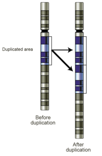
Schematic of a region of a chromosome before and after a duplication event

Replication slippage

Replication slippage is an error in DNA replication that can produce duplications of short genetic sequences. During replication DNA polymerase begins to copy the DNA. At some point during the replication process, the polymerase dissociates from the DNA and replication stalls. When the polymerase reattaches to the DNA strand, it aligns the replicating strand to an incorrect position and incidentally copies the same section more than once. Replication slippage is also often facilitated by repetitive sequences, but requires only a few bases of similarity.

Retrotransposition

Retrotransposons, mainly L1, can occasionally act on cellular mRNA. Transcripts are reverse transcribed to DNA and inserted into random place in the genome, creating retrogenes. Resulting sequence usually lack introns and often contain poly, sequences that are also integrated into the genome. Many retrogenes display changes in gene regulation in comparison to their parental gene sequences, which sometimes results in novel functions. Retrogenes can move between different chromosomes to shape chromosomal evolution.

Aneuploidy

Aneuploidy occurs when nondisjunction at a single chromosome results in an abnormal number of chromosomes. Aneuploidy is often harmful and in mammals regularly leads to spontaneous abortions (miscarriages). Some aneuploid individuals are viable, for example trisomy 21 in humans, which leads to Down syndrome. Aneuploidy often alters gene dosage in ways that are detrimental to the organism; therefore, it is unlikely to spread through populations.

Polyploidy

Polyploidy, or whole genome duplication is a product of nondisjunction during meiosis which results in additional copies of the entire genome. Polyploidy is common in plants, but it has also occurred in animals, with two rounds of whole genome duplication (2R event) in the vertebrate lineage leading to humans. It has also occurred in the hemiascomycete yeasts ~100 mya.

After a whole genome duplication, there is a relatively short period of genome instability, extensive gene loss, elevated levels of nucleotide substitution and regulatory network rewiring. In addition, gene dosage effects play a significant role. Thus, most duplicates are lost within a short period, however, a considerable fraction of duplicates survive. Interestingly, genes involved in regulation are preferentially retained. Furthermore, retention of regulatory genes, most notably the Hox genes, has led to adaptive innovation.

Rapid evolution and functional divergence have been observed at the level of the transcription of duplicated genes, usually by point mutations in short transcription factor binding motifs. Furthermore, rapid evolution of protein phosphorylation motifs, usually embedded within rapidly evolving intrinsically disordered regions is another contributing factor for survival and rapid adaptation/neofunctionalization of duplicate genes. Thus, a link seems to exist between gene regulation (at least at the post-translational level) and genome evolution.

Polyploidy is also a well known source of speciation, as offspring, which have different numbers of chromosomes compared to parent species, are often unable to interbreed with non-polyploid organisms. Whole genome duplications are thought to be less detrimental than aneuploidy as the relative dosage of individual genes should be the same.

As an evolutionary event

Evolutionary fate of duplicate genes

Rate of gene duplication

Comparisons of genomes demonstrate that gene duplications are common in most species investigated. This is indicated by variable copy numbers (copy number variation) in the genome of humans or fruit flies. However, it has been difficult to measure the rate at which such duplications occur. Recent studies yielded a first direct estimate of the genome-wide rate of gene duplication in C. elegans, the first multicellular eukaryote for which such as estimate became available. The gene duplication rate in C. elegans is on the order of 10⁻⁷ duplications/gene/generation, that is, in a population of 10 million worms, one will have a gene duplication per generation. This rate is two orders of magnitude greater than the spontaneous rate of point mutation per nucleotide site in this species. Older (indirect) studies reported locus-specific duplication rates in bacteria, Drosophila, and humans ranging from 10⁻³ to 10⁻⁷/gene/generation.

Neofunctionalization

Main article: Neofunctionalization

Gene duplications are an essential source of genetic novelty that can lead to evolutionary innovation. Duplication creates genetic redundancy, where the second copy of the gene is often free from selective pressure—that is, mutations of it have no deleterious effects to its host organism. If one copy of a gene experiences a mutation that affects its original function, the second copy can serve as a 'spare part' and continue to function correctly. Thus, duplicate genes accumulate mutations faster than a functional single-copy gene, over generations of organisms, and it is possible for one of the two copies to develop a new and different function. Some examples of such neofunctionalization is the apparent mutation of a duplicated digestive gene in a family of ice fish into an antifreeze gene and duplication leading to a novel snake venom gene and the synthesis of 1 beta-hydroxytestosterone in pigs.

Gene duplication is believed to play a major role in evolution; this stance has been held by members of the scientific community for over 100 years. Susumu Ohno was one of the most famous developers of this theory in his classic book Evolution by gene duplication (1970). Ohno argued that gene duplication is the most important evolutionary force since the emergence of the universal common ancestor. Major genome duplication events can be quite common. It is believed that the entire yeast genome underwent duplication about 100 million years ago. Plants are the most prolific genome duplicators. For example, wheat is hexaploid (a kind of polyploid), meaning that it has six copies of its genome.

Subfunctionalization

Main article: Subfunctionalization

Another possible fate for duplicate genes is that both copies are equally free to accumulate degenerative mutations, so long as any defects are complemented by the other copy. This leads to a neutral "subfunctionalization" (a process of constructive neutral evolution) or DDC (duplication-degeneration-complementation) model, in which the functionality of the original gene is distributed among the two copies. Neither gene can be lost, as both now perform important non-redundant functions, but ultimately neither is able to achieve novel functionality.

Subfunctionalization can occur through neutral processes in which mutations accumulate with no detrimental or beneficial effects. However, in some cases subfunctionalization can occur with clear adaptive benefits. If an ancestral gene is pleiotropic and performs two functions, often neither one of these two functions can be changed without affecting the other function. In this way, partitioning the ancestral functions into two separate genes can allow for adaptive specialization of subfunctions, thereby providing an adaptive benefit.

Loss

Often the resulting genomic variation leads to gene dosage dependent neurological disorders such as Rett-like syndrome and Pelizaeus–Merzbacher disease. Such detrimental mutations are likely to be lost from the population and will not be preserved or develop novel functions. However, many duplications are, in fact, not detrimental or beneficial, and these neutral sequences may be lost or may spread through the population through random fluctuations via genetic drift.

Identifying duplications in sequenced genomes

Criteria and single genome scans

The two genes that exist after a gene duplication event are called paralogs and usually code for proteins with a similar function and/or structure. By contrast, orthologous genes present in different species which are each originally derived from the same ancestral sequence. (See Homology of sequences in genetics).

It is important (but often difficult) to differentiate between paralogs and orthologs in biological research. Experiments on human gene function can often be carried out on other species if a homolog to a human gene can be found in the genome of that species, but only if the homolog is orthologous. If they are paralogs and resulted from a gene duplication event, their functions are likely to be too different. One or more copies of duplicated genes that constitute a gene family may be affected by insertion of transposable elements that causes significant variation between them in their sequence and finally may become responsible for divergent evolution. This may also render the chances and the rate of gene conversion between the homologs of gene duplicates due to less or no similarity in their sequences.

Paralogs can be identified in single genomes through a sequence comparison of all annotated gene models to one another. Such a comparison can be performed on translated amino acid sequences (e.g. BLASTp, tBLASTx) to identify ancient duplications or on DNA nucleotide sequences (e.g. BLASTn, megablast) to identify more recent duplications. Most studies to identify gene duplications require reciprocal-best-hits or fuzzy reciprocal-best-hits, where each paralog must be the other's single best match in a sequence comparison.

Most gene duplications exist as low copy repeats (LCRs), rather highly repetitive sequences like transposable elements. They are mostly found in pericentronomic, subtelomeric and interstitial regions of a chromosome. Many LCRs, due to their size (>1Kb), similarity, and orientation, are highly susceptible to duplications and deletions.

Genomic microarrays detect duplications

Technologies such as genomic microarrays, also called array comparative genomic hybridization (array CGH), are used to detect chromosomal abnormalities, such as microduplications, in a high throughput fashion from genomic DNA samples. In particular, DNA microarray technology can simultaneously monitor the expression levels of thousands of genes across many treatments or experimental conditions, greatly facilitating the evolutionary studies of gene regulation after gene duplication or speciation.

Next generation sequencing

Gene duplications can also be identified through the use of next-generation sequencing platforms. The simplest means to identify duplications in genomic resequencing data is through the use of paired-end sequencing reads. Tandem duplications are indicated by sequencing read pairs which map in abnormal orientations. Through a combination of increased sequence coverage and abnormal mapping orientation, it is possible to identify duplications in genomic sequencing data.

Nomenclature

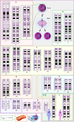
Human karyotype with annotated bands and sub-bands as used for the nomenclature of chromosome abnormalities. It shows dark and white regions as seen on G banding. Each row is vertically aligned at centromere level. It shows 22 homologous autosomal chromosome pairs, both the female (XX) and male (XY) versions of the two sex chromosomes, as well as the mitochondrial genome (at bottom left).

Further information: Karyotype

The International System for Human Cytogenomic Nomenclature (ISCN) is an international standard for human chromosome nomenclature, which includes band names, symbols and abbreviated terms used in the description of human chromosome and chromosome abnormalities. Abbreviations include dup for duplications of parts of a chromosome. For example, dup(17p12) causes Charcot–Marie–Tooth disease type 1A.

As amplification

Gene duplication does not necessarily constitute a lasting change in a species' genome. In fact, such changes often don't last past the initial host organism. From the perspective of molecular genetics, gene amplification is one of many ways in which a gene can be overexpressed. Genetic amplification can occur artificially, as with the use of the polymerase chain reaction technique to amplify short strands of DNA in vitro using enzymes, or it can occur naturally, as described above. If it's a natural duplication, it can still take place in a somatic cell, rather than a germline cell (which would be necessary for a lasting evolutionary change).

Role in cancer

Duplications of oncogenes are a common cause of many types of cancer. In such cases the genetic duplication occurs in a somatic cell and affects only the genome of the cancer cells themselves, not the entire organism, much less any subsequent offspring. Recent comprehensive patient-level classification and quantification of driver events in TCGA cohorts revealed that there are on average 12 driver events per tumor, of which 1.5 are amplifications of oncogenes.

Common oncogene amplifications in human cancers

Cancer type	Associated gene amplifications	Prevalence of amplification in cancer type (percent)
Breast cancer	MYC	20%
	ERBB2 (HER2)	20%
	CCND1 (Cyclin D1)	15–20%
	FGFR1	12%
	FGFR2	12%
Cervical cancer	MYC	25–50%
	ERBB2	20%
Colorectal cancer	HRAS	30%
	KRAS	20%
	MYB	15–20%
Esophageal cancer	MYC	40%
	CCND1	25%
	MDM2	13%
Gastric cancer	CCNE (Cyclin E)	15%
	KRAS	10%
	MET	10%
Glioblastoma	ERBB1 (EGFR)	33–50%
	CDK4	15%
Head and neck cancer	CCND1	50%
	ERBB1	10%
	MYC	7–10%
Hepatocellular cancer	CCND1	13%
Neuroblastoma	MYCN	20–25%
Ovarian cancer	MYC	20–30%
	ERBB2	15–30%
	AKT2	12%
Sarcoma	MDM2	10–30%
	CDK4	10%
Small cell lung cancer	MYC	15–20%

Whole-genome duplications are also frequent in cancers, detected in 30% to 36% of tumors from the most common cancer types. Their exact role in carcinogenesis is unclear, but they in some cases lead to loss of chromatin segregation leading to chromatin conformation changes that in turn lead to oncogenic epigenetic and transcriptional modifications.

Enzyme promiscuity

From Wikipedia, the free encyclopedia

Enzyme promiscuity is the ability of an enzyme to catalyse a fortuitous side reaction in addition to its main reaction. Although enzymes are remarkably specific catalysts, they can often perform side reactions in addition to their main, native catalytic activity. These promiscuous activities are usually slow relative to the main activity and are under neutral selection. Despite ordinarily being physiologically irrelevant, under new selective pressures these activities may confer a fitness benefit therefore prompting the evolution of the formerly promiscuous activity to become the new main activity. An example of this is the atrazine chlorohydrolase (atzA encoded) from Pseudomonas sp. ADP that evolved from melamine deaminase (triA encoded), which has very small promiscuous activity toward atrazine, a man-made chemical.

Introduction

Enzymes are evolved to catalyse a particular reaction on a particular substrate with a high catalytic efficiency (k_cat/K_M, cf. Michaelis–Menten kinetics). However, in addition to this main activity, they possess other activities that are generally several orders of magnitude lower, and that are not a result of evolutionary selection and therefore do not partake in the physiology of the organism. This phenomenon allows new functions to be gained as the promiscuous activity could confer a fitness benefit under a new selective pressure leading to its duplication and selection as a new main activity.

Enzyme evolution

Duplication and divergence

Several theoretical models exist to predict the order of duplication and specialisation events, but the actual process is more intertwined and fuzzy (§ Reconstructed enzymes below). On one hand, gene amplification results in an increase in enzyme concentration, and potentially freedom from a restrictive regulation, therefore increasing the reaction rate (v) of the promiscuous activity of the enzyme making its effects more pronounced physiologically ("gene dosage effect"). On the other, enzymes may evolve an increased secondary activity with little loss to the primary activity ("robustness") with little adaptive conflict (§ Robustness and plasticity below).

Robustness and plasticity

A study of four distinct hydrolases (human serum paraoxonase (PON1), pseudomonad phosphotriesterase (PTE), Protein tyrosine phospatase(PTP) and human carbonic anhydrase II (CAII)) has shown the main activity is "robust" towards change, whereas the promiscuous activities are weak and more "plastic". Specifically, selecting for an activity that is not the main activity (via directed evolution), does not initially diminish the main activity (hence its robustness), but greatly affects the non-selected activities (hence their plasticity).

The phosphotriesterase (PTE) from Pseudomonas diminuta was evolved to become an arylesterase (P–O to C–O hydrolase) in eighteen rounds gaining a 10⁹ shift in specificity (ratio of K_M), however most of the change occurred in the initial rounds, where the unselected vestigial PTE activity was retained and the evolved arylesterase activity grew, while in the latter rounds there was a little trade-off for the loss of the vestigial PTE activity in favour of the arylesterase activity.

This means firstly that a specialist enzyme (monofunctional) when evolved goes through a generalist stage (multifunctional), before becoming a specialist again—presumably after gene duplication according to the IAD model—and secondly that promiscuous activities are more plastic than the main activity.

Reconstructed enzymes

The most recent and most clear cut example of enzyme evolution is the rise of bioremediating enzymes in the past 60 years. Due to the very low number of amino acid changes, these provide an excellent model to investigate enzyme evolution in nature. However, using extant enzymes to determine how the family of enzymes evolved has the drawback that the newly evolved enzyme is compared to paralogues without knowing the true identity of the ancestor before the two genes diverged. This issue can be resolved thanks to ancestral reconstruction. First proposed in 1963 by Linus Pauling and Emile Zuckerkandl, ancestral reconstruction is the inference and synthesis of a gene from the ancestral form of a group of genes, which has had a recent revival thanks to improved inference techniques and low-cost artificial gene synthesis, resulting in several ancestral enzymes—dubbed "stemzymes" by some—to be studied.

Evidence gained from reconstructed enzyme suggests that the order of the events where the novel activity is improved and the gene is duplication is not clear cut, unlike what the theoretical models of gene evolution suggest.

One study showed that the ancestral gene of the immune defence protease family in mammals had a broader specificity and a higher catalytic efficiency than the contemporary family of paralogues, whereas another study showed that the ancestral steroid receptor of vertebrates was an oestrogen receptor with slight substrate ambiguity for other hormones—indicating that these probably were not synthesised at the time.

This variability in ancestral specificity has not only been observed between different genes, but also within the same gene family. In light of the large number of paralogous fungal α-glucosidase genes with a number of specific maltose-like (maltose, turanose, maltotriose, maltulose and sucrose) and isomaltose-like (isomaltose and palatinose) substrates, a study reconstructed all key ancestors and found that the last common ancestor of the paralogues was mainly active on maltose-like substrates with only trace activity for isomaltose-like sugars, despite leading to a lineage of iso-maltose glucosidases and a lineage that further split into maltose glucosidases and iso-maltose glucosidases. Antithetically, the ancestor before the latter split had a more pronounced isomaltose-like glucosidase activity.

Primordial metabolism

Roy Jensen in 1976 theorised that primordial enzymes had to be highly promiscuous in order for metabolic networks to assemble in a patchwork fashion (hence its name, the patchwork model). This primordial catalytic versatility was later lost in favour of highly catalytic specialised orthologous enzymes. As a consequence, many central-metabolic enzymes have structural homologues that diverged before the last universal common ancestor.

Distribution

Promiscuity is not only a primordial trait, but also a very widespread property in modern genomes. A series of experiments have been conducted to assess the distribution of promiscuous enzyme activities in E. coli. In E. coli 21 out of 104 single-gene knockouts tested (from the Keio collection) could be rescued by overexpressing a noncognate E. coli protein (using a pooled set of plasmids of the ASKA collection). The mechanisms by which the noncognate ORF could rescue the knockout can be grouped into eight categories: isozyme overexpression (homologues), substrate ambiguity, transport ambiguity (scavenging), catalytic promiscuity, metabolic flux maintenance (including overexpression of the large component of a synthase in the absence of the amine transferase subunit), pathway bypass, regulatory effects and unknown mechanisms. Similarly, overexpressing the ORF collection allowed E. coli to gain over an order of magnitude in resistance in 86 out 237 toxic environment.

Homology

Homologues are sometimes known to display promiscuity towards each other's main reactions. This crosswise promiscuity has been most studied with members of the alkaline phosphatase superfamily, which catalyse hydrolytic reaction on the sulfate, phosphonate, monophosphate, diphosphate or triphosphate ester bond of several compounds. Despite the divergence the homologues have a varying degree of reciprocal promiscuity: the differences in promiscuity are due to mechanisms involved, particularly the intermediate required.

Degree of promiscuity

Enzymes are generally in a state that is not only a compromise between stability and catalytic efficiency, but also for specificity and evolvability, the latter two dictating whether an enzyme is a generalist (highly evolvable due to large promiscuity, but low main activity) or a specialist (high main activity, poorly evolvable due to low promiscuity). Examples of these are enzymes for primary and secondary metabolism in plants (§ Plant secondary metabolism below). Other factors can come into play, for example the glycerophosphodiesterase (gpdQ) from Enterobacter aerogenes shows different values for its promiscuous activities depending on the two metal ions it binds, which is dictated by ion availability. some cases promiscuity can be increased by relaxing the specificity of the active site by enlarging it with a single mutation as was the case of a D297G mutant of the E. coli L-Ala-D/L-Glu epimerase (ycjG) and E323G mutant of a pseudomonad muconate lactonizing enzyme II, allowing them to promiscuously catalyse the activity of O-succinylbenzoate synthase (menC). Conversely, promiscuity can be decreased as was the case of γ-humulene synthase (a sesquiterpene synthase) from Abies grandis that is known to produce 52 different sesquiterpenes from farnesyl diphosphate upon several mutations.

Studies on enzymes with broad-specificity—not promiscuous, but conceptually close—such as mammalian trypsin and chymotrypsin, and the bifunctional isopropylmalate isomerase/homoaconitase from Pyrococcus horikoshii have revealed that active site loop mobility contributes substantially to the catalytic elasticity of the enzyme.

Toxicity

A promiscuous activity is a non-native activity the enzyme did not evolve to do, but arises due to an accommodating conformation of the active site. However, the main activity of the enzyme is a result not only of selection towards a high catalytic rate towards a particular substrate to produce a particular product, but also to avoid the production of toxic or unnecessary products. For example, if a tRNA syntheses loaded an incorrect amino acid onto a tRNA, the resulting peptide would have unexpectedly altered properties, consequently to enhance fidelity several additional domains are present. Similar in reaction to tRNA syntheses, the first subunit of tyrocidine synthetase (tyrA) from Bacillus brevis adenylates a molecule of phenylalanine in order to use the adenyl moiety as a handle to produce tyrocidine, a cyclic non-ribosomal peptide. When the specificity of enzyme was probed, it was found that it was highly selective against natural amino acids that were not phenylalanine, but was much more tolerant towards unnatural amino acids. Specifically, most amino acids were not catalysed, whereas the next most catalysed native amino acid was the structurally similar tyrosine, but at a thousandth as much as phenylalanine, whereas several unnatural amino acids where catalysed better than tyrosine, namely D-phenylalanine, β-cyclohexyl-L-alanine, 4-amino-L-phenylalanine and L-norleucine.

One peculiar case of selected secondary activity are polymerases and restriction endonucleases, where incorrect activity is actually a result of a compromise between fidelity and evolvability. For example, for restriction endonucleases incorrect activity (star activity) is often lethal for the organism, but a small amount allows new functions to evolve against new pathogens.

Plant secondary metabolism

Anthocyanins (delphinidin pictured) confer plants, particularly their flowers, with a variety of colours to attract pollinators and a typical example of plant secondary metabolite.

Plants produce a large number of secondary metabolites thanks to enzymes that, unlike those involved in primary metabolism, are less catalytically efficient but have a larger mechanistic elasticity (reaction types) and broader specificities. The liberal drift threshold (caused by the low selective pressure due to the small population size) allows the fitness gain endowed by one of the products to maintain the other activities even though they may be physiologically useless.

Biocatalysis

Main article: biocatalysis

In biocatalysis, many reactions are sought that are absent in nature. To do this, enzymes with a small promiscuous activity towards the required reaction are identified and evolved via directed evolution or rational design.

An example of a commonly evolved enzyme is ω-transaminase which can replace a ketone with a chiral amine and consequently libraries of different homologues are commercially available for rapid biomining (eg. Codexis).

Another example is the possibility of using the promiscuous activities of cysteine synthase (cysM) towards nucleophiles to produce non-proteinogenic amino acids.

Reaction similarity

Similarity between enzymatic reactions (EC) can be calculated by using bond changes, reaction centres or substructure metrics (EC-BLAST Archived 2019-05-30 at the Wayback Machine).

Drugs and promiscuity

Whereas promiscuity is mainly studied in terms of standard enzyme kinetics, drug binding and subsequent reaction is a promiscuous activity as the enzyme catalyses an inactivating reaction towards a novel substrate it did not evolve to catalyse. This could be because of the demonstration that there are only a small number of distinct ligand binding pockets in proteins.

Mammalian xenobiotic metabolism, on the other hand, was evolved to have a broad specificity to oxidise, bind and eliminate foreign lipophilic compounds which may be toxic, such as plant alkaloids, so their ability to detoxify anthropogenic xenobiotics is an extension of this.

Data structure

From Wikipedia, the free encyclopedia

https://en.wikipedia.org/wiki/Data_structure 

 

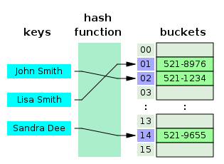
A data structure known as a hash table.

In computer science, a data structure is a data organization, management, and storage format that is usually chosen for efficient access to data. More precisely, a data structure is a collection of data values, the relationships among them, and the functions or operations that can be applied to the data, i.e., it is an algebraic structure about data.

Usage

Data structures serve as the basis for abstract data types (ADT). The ADT defines the logical form of the data type. The data structure implements the physical form of the data type.

Different types of data structures are suited to different kinds of applications, and some are highly specialized to specific tasks. For example, relational databases commonly use B-tree indexes for data retrieval, while compiler implementations usually use hash tables to look up identifiers.

Data structures provide a means to manage large amounts of data efficiently for uses such as large databases and internet indexing services. Usually, efficient data structures are key to designing efficient algorithms. Some formal design methods and programming languages emphasize data structures, rather than algorithms, as the key organizing factor in software design. Data structures can be used to organize the storage and retrieval of information stored in both main memory and secondary memory.

Implementation

Data structures can be implemented using a variety of programming languages and techniques, but they all share the common goal of efficiently organizing and storing data. Data structures are generally based on the ability of a computer to fetch and store data at any place in its memory, specified by a pointer—a bit string, representing a memory address, that can be itself stored in memory and manipulated by the program. Thus, the array and record data structures are based on computing the addresses of data items with arithmetic operations, while the linked data structures are based on storing addresses of data items within the structure itself. This approach to data structuring has profound implications for the efficiency and scalability of algorithms. For instance, the contiguous memory allocation in arrays facilitates rapid access and modification operations, leading to optimized performance in sequential data processing scenarios.

The implementation of a data structure usually requires writing a set of procedures that create and manipulate instances of that structure. The efficiency of a data structure cannot be analyzed separately from those operations. This observation motivates the theoretical concept of an abstract data type, a data structure that is defined indirectly by the operations that may be performed on it, and the mathematical properties of those operations (including their space and time cost).

Examples

Main article: List of data structures

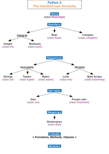
The standard type hierarchy of the programming language Python 3.

There are numerous types of data structures, generally built upon simpler primitive data types. Well known examples are:

• An array is a number of elements in a specific order, typically all of the same type (depending on the language, individual elements may either all be forced to be the same type, or may be of almost any type). Elements are accessed using an integer index to specify which element is required. Typical implementations allocate contiguous memory words for the elements of arrays (but this is not always a necessity). Arrays may be fixed-length or resizable.
• A linked list (also just called list) is a linear collection of data elements of any type, called nodes, where each node has itself a value, and points to the next node in the linked list. The principal advantage of a linked list over an array is that values can always be efficiently inserted and removed without relocating the rest of the list. Certain other operations, such as random access to a certain element, are however slower on lists than on arrays.
• A record (also called tuple or struct) is an aggregate data structure. A record is a value that contains other values, typically in fixed number and sequence and typically indexed by names. The elements of records are usually called fields or members. In the context of object-oriented programming, records are known as plain old data structures to distinguish them from objects.
• Hash tables, also known as hash maps, are data structures that provide fast retrieval of values based on keys. They use a hashing function to map keys to indexes in an array, allowing for constant-time access in the average case. Hash tables are commonly used in dictionaries, caches, and database indexing. However, hash collisions can occur, which can impact their performance. Techniques like chaining and open addressing are employed to handle collisions.
• Graphs are collections of nodes connected by edges, representing relationships between entities. Graphs can be used to model social networks, computer networks, and transportation networks, among other things. They consist of vertices (nodes) and edges (connections between nodes). Graphs can be directed or undirected, and they can have cycles or be acyclic. Graph traversal algorithms include breadth-first search and depth-first search.
• Stacks and queues are abstract data types that can be implemented using arrays or linked lists. A stack has two primary operations: push (adds an element to the top of the stack) and pop (removes the topmost element from the stack), that follow the Last In, First Out (LIFO) principle. Queues have two main operations: enqueue (adds an element to the rear of the queue) and dequeue (removes an element from the front of the queue) that follow the First In, First Out (FIFO) principle.
• Trees represent a hierarchical organization of elements. A tree consists of nodes connected by edges, with one node being the root and all other nodes forming subtrees. Trees are widely used in various algorithms and data storage scenarios. Binary trees (particularly heaps), AVL trees, and B-trees are some popular types of trees. They enable efficient and optimal searching, sorting, and hierarchical representation of data.
• A trie, also known as a prefix tree, is a specialized tree data structure used for the efficient retrieval of strings. Tries store characters of a string as nodes, with each edge representing a character. They are particularly useful in text processing scenarios like autocomplete, spell-checking, and dictionary implementations. Tries enable fast searching and prefix-based operations on strings.

Language support

Most assembly languages and some low-level languages, such as BCPL (Basic Combined Programming Language), lack built-in support for data structures. On the other hand, many high-level programming languages and some higher-level assembly languages, such as MASM, have special syntax or other built-in support for certain data structures, such as records and arrays. For example, the C (a direct descendant of BCPL) and Pascal languages support structs and records, respectively, in addition to vectors (one-dimensional arrays) and multi-dimensional arrays.

Most programming languages feature some sort of library mechanism that allows data structure implementations to be reused by different programs. Modern languages usually come with standard libraries that implement the most common data structures. Examples are the C++ Standard Template Library, the Java Collections Framework, and the Microsoft .NET Framework.

Modern languages also generally support modular programming, the separation between the interface of a library module and its implementation. Some provide opaque data types that allow clients to hide implementation details. Object-oriented programming languages, such as C++, Java, and Smalltalk, typically use classes for this purpose.

Low-level programming language

From Wikipedia, the free encyclopedia
https://en.wikipedia.org/wiki/Low-level_programming_language

A low-level programming language is a programming language that provides little or no abstraction from a computer's instruction set architecture—commands or functions in the language map that are structurally similar to processor's instructions. Generally, this refers to either machine code or assembly language. Because of the low (hence the word) abstraction between the language and machine language, low-level languages are sometimes described as being "close to the hardware". Programs written in low-level languages tend to be relatively non-portable, due to being optimized for a certain type of system architecture.

Low-level languages can convert to machine code without a compiler or interpreter—second-generation programming languages use a simpler processor called an assembler—and the resulting code runs directly on the processor. A program written in a low-level language can be made to run very quickly, with a small memory footprint. An equivalent program in a high-level language can be less efficient and use more memory. Low-level languages are simple, but considered difficult to use, due to numerous technical details that the programmer must remember. By comparison, a high-level programming language isolates execution semantics of a computer architecture from the specification of the program, which simplifies development.

Machine code

Front panel of a PDP-8/E minicomputer. The row of switches at the bottom can be used to toggle in a machine language program.

Main article: Machine code

Machine code is the only language a computer can process directly without a previous transformation. Currently, programmers almost never write programs directly in machine code, because it requires attention to numerous details that a high-level programming language handles automatically. Furthermore, unlike programming in an assembly language, it requires memorizing or looking up numerical codes for every instruction, and is extremely difficult to modify.

True machine code is a stream of raw, usually binary, data. A programmer coding in "machine code" normally codes instructions and data in a more readable form such as decimal, octal, or hexadecimal which is translated to internal format by a program called a loader or toggled into the computer's memory from a front panel.

Although few programs are written in machine languages, programmers often become adept at reading it through working with core dumps or debugging from the front panel.

Example of a function in hexadecimal representation of x86-64 machine code to calculate the nth Fibonacci number, with each line corresponding to one instruction:

89 f8
85 ff
74 26
83 ff 02
76 1c
89 f9
ba 01 00 00 00
be 01 00 00 00
8d 04 16
83 f9 02
74 0d
89 d6
ff c9
89 c2
eb f0
b8 01 00 00
c3

Assembly language

Main article: Assembly language

Second-generation languages provide one abstraction level on top of the machine code. In the early days of coding on computers like TX-0 and PDP-1, the first thing MIT hackers did was to write assemblers. Assembly language has little semantics or formal specification, being only a mapping of human-readable symbols, including symbolic addresses, to opcodes, addresses, numeric constants, strings and so on. Typically, one machine instruction is represented as one line of assembly code. Assemblers produce object files that can link with other object files or be loaded on their own.

Most assemblers provide macros to generate common sequences of instructions.

Example: The same Fibonacci number calculator as above, but in x86-64 assembly language using AT&T syntax:

fib:
        movl %edi, %eax        ; put the argument into %eax
        testl %edi, %edi       ; is it zero?
        je .return_from_fib    ; yes - return 0, which is already in %eax
        cmpl $2, %edi          ; is 2 greater than or equal to it?
        jbe .return_1_from_fib ; yes (i.e., it's 1 or 2) - return 1
        movl %edi, %ecx        ; no - put it in %ecx, for use as a counter
        movl $1, %edx          ; the previous number in the sequence, which starts out as 1
        movl $1, %esi          ; the number before that, which also starts out as 1
.fib_loop:
        leal (%rsi,%rdx), %eax ; put the sum of the previous two numbers into %eax
        cmpl $2, %ecx          ; is the counter 2?
        je .return_from_fib    ; yes - %eax contains the result
        movl %edx, %esi        ; make the previous number the number before the previous one
        decl %ecx              ; decrement the counter
        movl %eax, %edx        ; make the current number the previous number
        jmp .fib_loop          ; keep going
.return_1_from_fib:
        movl $1, %eax          ; set the return value to 1
.return_from_fib:
        ret                    ; return

In this code example, the registers of the x86-64 processor are named and manipulated directly. The function loads its 32-bit argument from %edi in accordance to the System V application binary interface for x86-64 and performs its calculation by manipulating values in the %eax, %ecx, %esi, and %edi registers until it has finished and returns. Note that in this assembly language, there is no concept of returning a value. The result having been stored in the %eax register, again in accordance with System V application binary interface, the ret instruction simply removes the top 64-bit element on the stack and causes the next instruction to be fetched from that location (that instruction is usually the instruction immediately after the one that called this function), with the result of the function being stored in %eax. x86-64 assembly language imposes no standard for passing values to a function or returning values from a function (and in fact, has no concept of a function); those are defined by an application binary interface, such as the System V ABI for a particular instruction set.

Compare this with the same function in C:

unsigned int fib(unsigned int n) {
   if (!n)
       return 0;
   else if (n <= 2)
       return 1;
   else {
       unsigned int f_nminus2, f_nminus1, f_n;       
       for (f_nminus2 = f_nminus1 = 1, f_n = 0; ; --n) {
           f_n = f_nminus2 + f_nminus1;
           if (n <= 2) return f_n;
           f_nminus2 = f_nminus1;
       }
   }
}

This code is similar in structure to the assembly language example but there are significant differences in terms of abstraction:

• The input (parameter n) is an abstraction that does not specify any storage location on the hardware. In practice, the C compiler follows one of many possible calling conventions to determine a storage location for the input.
• The local variables f_nminus2, f_nminus2, and f_n are abstractions that do not specify any specific storage location on the hardware. The C compiler decides how to actually store them for the target architecture.
• The return function specifies the value to return, but does not dictate how it is returned. The C compiler for any specific architecture implements a standard mechanism for returning the value. Compilers for the x86 architecture typically (but not always) use the %eax register to return a value, as in the assembly language example (the author of the assembly language example has chosen to use the System V application binary interface for x86-64 convention but assembly language does not require this).

These abstractions make the C code compilable without modification on any architecture for which a C compiler has been written. The x86 assembly language code is specific to the x86-64 architecture and the System V application binary interface for that architecture.

Low-level programming in high-level languages

During the late 1960s and 1970s, high-level languages that included some degree of access to low-level programming functions, such as PL/S, BLISS, BCPL, extended ALGOL and ESPOL (for Burroughs large systems), and C, were introduced. One method for this is inline assembly, in which assembly code is embedded in a high-level language that supports this feature. Some of these languages also allow architecture-dependent compiler optimization directives to adjust the way a compiler uses the target processor architecture.