Search This Blog

Saturday, December 23, 2023

Economic model

From Wikipedia, the free encyclopedia

An economic model is a theoretical construct representing economic processes by a set of variables and a set of logical and/or quantitative relationships between them. The economic model is a simplified, often mathematical, framework designed to illustrate complex processes. Frequently, economic models posit structural parameters. A model may have various exogenous variables, and those variables may change to create various responses by economic variables. Methodological uses of models include investigation, theorizing, and fitting theories to the world.

Overview

In general terms, economic models have two functions: first as a simplification of and abstraction from observed data, and second as a means of selection of data based on a paradigm of econometric study.

Simplification is particularly important for economics given the enormous complexity of economic processes. This complexity can be attributed to the diversity of factors that determine economic activity; these factors include: individual and cooperative decision processes, resource limitations, environmental and geographical constraints, institutional and legal requirements and purely random fluctuations. Economists therefore must make a reasoned choice of which variables and which relationships between these variables are relevant and which ways of analyzing and presenting this information are useful.

Selection is important because the nature of an economic model will often determine what facts will be looked at and how they will be compiled. For example, inflation is a general economic concept, but to measure inflation requires a model of behavior, so that an economist can differentiate between changes in relative prices and changes in price that are to be attributed to inflation.

In addition to their professional academic interest, uses of models include:

  • Forecasting economic activity in a way in which conclusions are logically related to assumptions;
  • Proposing economic policy to modify future economic activity;
  • Presenting reasoned arguments to politically justify economic policy at the national level, to explain and influence company strategy at the level of the firm, or to provide intelligent advice for household economic decisions at the level of households.
  • Planning and allocation, in the case of centrally planned economies, and on a smaller scale in logistics and management of businesses.
  • In finance, predictive models have been used since the 1980s for trading (investment and speculation). For example, emerging market bonds were often traded based on economic models predicting the growth of the developing nation issuing them. Since the 1990s many long-term risk management models have incorporated economic relationships between simulated variables in an attempt to detect high-exposure future scenarios (often through a Monte Carlo method).

A model establishes an argumentative framework for applying logic and mathematics that can be independently discussed and tested and that can be applied in various instances. Policies and arguments that rely on economic models have a clear basis for soundness, namely the validity of the supporting model.

Economic models in current use do not pretend to be theories of everything economic; any such pretensions would immediately be thwarted by computational infeasibility and the incompleteness or lack of theories for various types of economic behavior. Therefore, conclusions drawn from models will be approximate representations of economic facts. However, properly constructed models can remove extraneous information and isolate useful approximations of key relationships. In this way more can be understood about the relationships in question than by trying to understand the entire economic process.

The details of model construction vary with type of model and its application, but a generic process can be identified. Generally, any modelling process has two steps: generating a model, then checking the model for accuracy (sometimes called diagnostics). The diagnostic step is important because a model is only useful to the extent that it accurately mirrors the relationships that it purports to describe. Creating and diagnosing a model is frequently an iterative process in which the model is modified (and hopefully improved) with each iteration of diagnosis and respecification. Once a satisfactory model is found, it should be double checked by applying it to a different data set.

Types of models

According to whether all the model variables are deterministic, economic models can be classified as stochastic or non-stochastic models; according to whether all the variables are quantitative, economic models are classified as discrete or continuous choice model; according to the model's intended purpose/function, it can be classified as quantitative or qualitative; according to the model's ambit, it can be classified as a general equilibrium model, a partial equilibrium model, or even a non-equilibrium model; according to the economic agent's characteristics, models can be classified as rational agent models, representative agent models etc.

  • Stochastic models are formulated using stochastic processes. They model economically observable values over time. Most of econometrics is based on statistics to formulate and test hypotheses about these processes or estimate parameters for them. A widely used bargaining class of simple econometric models popularized by Tinbergen and later Wold are autoregressive models, in which the stochastic process satisfies some relation between current and past values. Examples of these are autoregressive moving average models and related ones such as autoregressive conditional heteroskedasticity (ARCH) and GARCH models for the modelling of heteroskedasticity.
  • Non-stochastic models may be purely qualitative (for example, relating to social choice theory) or quantitative (involving rationalization of financial variables, for example with hyperbolic coordinates, and/or specific forms of functional relationships between variables). In some cases economic predictions in a coincidence of a model merely assert the direction of movement of economic variables, and so the functional relationships are used only stoical in a qualitative sense: for example, if the price of an item increases, then the demand for that item will decrease. For such models, economists often use two-dimensional graphs instead of functions.
  • Qualitative models – although almost all economic models involve some form of mathematical or quantitative analysis, qualitative models are occasionally used. One example is qualitative scenario planning in which possible future events are played out. Another example is non-numerical decision tree analysis. Qualitative models often suffer from lack of precision.

At a more practical level, quantitative modelling is applied to many areas of economics and several methodologies have evolved more or less independently of each other. As a result, no overall model taxonomy is naturally available. We can nonetheless provide a few examples that illustrate some particularly relevant points of model construction.

  • An accounting model is one based on the premise that for every credit there is a debit. More symbolically, an accounting model expresses some principle of conservation in the form
algebraic sum of inflows = sinks − sources
This principle is certainly true for money and it is the basis for national income accounting. Accounting models are true by convention, that is any experimental failure to confirm them, would be attributed to fraud, arithmetic error or an extraneous injection (or destruction) of cash, which we would interpret as showing the experiment was conducted improperly.
  • Optimality and constrained optimization models – Other examples of quantitative models are based on principles such as profit or utility maximization. An example of such a model is given by the comparative statics of taxation on the profit-maximizing firm. The profit of a firm is given by
where is the price that a product commands in the market if it is supplied at the rate , is the revenue obtained from selling the product, is the cost of bringing the product to market at the rate , and is the tax that the firm must pay per unit of the product sold.
The profit maximization assumption states that a firm will produce at the output rate x if that rate maximizes the firm's profit. Using differential calculus we can obtain conditions on x under which this holds. The first order maximization condition for x is
Regarding x as an implicitly defined function of t by this equation (see implicit function theorem), one concludes that the derivative of x with respect to t has the same sign as
which is negative if the second order conditions for a local maximum are satisfied.
Thus the profit maximization model predicts something about the effect of taxation on output, namely that output decreases with increased taxation. If the predictions of the model fail, we conclude that the profit maximization hypothesis was false; this should lead to alternate theories of the firm, for example based on bounded rationality.
Borrowing a notion apparently first used in economics by Paul Samuelson, this model of taxation and the predicted dependency of output on the tax rate, illustrates an operationally meaningful theorem; that is one requiring some economically meaningful assumption that is falsifiable under certain conditions.
  • Aggregate models. Macroeconomics needs to deal with aggregate quantities such as output, the price level, the interest rate and so on. Now real output is actually a vector of goods and services, such as cars, passenger airplanes, computers, food items, secretarial services, home repair services etc. Similarly price is the vector of individual prices of goods and services. Models in which the vector nature of the quantities is maintained are used in practice, for example Leontief input–output models are of this kind. However, for the most part, these models are computationally much harder to deal with and harder to use as tools for qualitative analysis. For this reason, macroeconomic models usually lump together different variables into a single quantity such as output or price. Moreover, quantitative relationships between these aggregate variables are often parts of important macroeconomic theories. This process of aggregation and functional dependency between various aggregates usually is interpreted statistically and validated by econometrics. For instance, one ingredient of the Keynesian model is a functional relationship between consumption and national income: C = C(Y). This relationship plays an important role in Keynesian analysis.

Problems with economic models

Most economic models rest on a number of assumptions that are not entirely realistic. For example, agents are often assumed to have perfect information, and markets are often assumed to clear without friction. Or, the model may omit issues that are important to the question being considered, such as externalities. Any analysis of the results of an economic model must therefore consider the extent to which these results may be compromised by inaccuracies in these assumptions, and a large literature has grown up discussing problems with economic models, or at least asserting that their results are unreliable.

History

One of the major problems addressed by economic models has been understanding economic growth. An early attempt to provide a technique to approach this came from the French physiocratic school in the eighteenth century. Among these economists, François Quesnay was known particularly for his development and use of tables he called Tableaux économiques. These tables have in fact been interpreted in more modern terminology as a Leontiev model, see the Phillips reference below.

All through the 18th century (that is, well before the founding of modern political economy, conventionally marked by Adam Smith's 1776 Wealth of Nations), simple probabilistic models were used to understand the economics of insurance. This was a natural extrapolation of the theory of gambling, and played an important role both in the development of probability theory itself and in the development of actuarial science. Many of the giants of 18th century mathematics contributed to this field. Around 1730, De Moivre addressed some of these problems in the 3rd edition of The Doctrine of Chances. Even earlier (1709), Nicolas Bernoulli studies problems related to savings and interest in the Ars Conjectandi. In 1730, Daniel Bernoulli studied "moral probability" in his book Mensura Sortis, where he introduced what would today be called "logarithmic utility of money" and applied it to gambling and insurance problems, including a solution of the paradoxical Saint Petersburg problem. All of these developments were summarized by Laplace in his Analytical Theory of Probabilities (1812). Thus, by the time David Ricardo came along he had a well-established mathematical basis to draw from.

Tests of macroeconomic predictions

In the late 1980s, the Brookings Institution compared 12 leading macroeconomic models available at the time. They compared the models' predictions for how the economy would respond to specific economic shocks (allowing the models to control for all the variability in the real world; this was a test of model vs. model, not a test against the actual outcome). Although the models simplified the world and started from a stable, known common parameters the various models gave significantly different answers. For instance, in calculating the impact of a monetary loosening on output some models estimated a 3% change in GDP after one year, and one gave almost no change, with the rest spread between.

Partly as a result of such experiments, modern central bankers no longer have as much confidence that it is possible to 'fine-tune' the economy as they had in the 1960s and early 1970s. Modern policy makers tend to use a less activist approach, explicitly because they lack confidence that their models will actually predict where the economy is going, or the effect of any shock upon it. The new, more humble, approach sees danger in dramatic policy changes based on model predictions, because of several practical and theoretical limitations in current macroeconomic models; in addition to the theoretical pitfalls, (listed above) some problems specific to aggregate modelling are:

  • Limitations in model construction caused by difficulties in understanding the underlying mechanisms of the real economy. (Hence the profusion of separate models.)
  • The law of unintended consequences, on elements of the real economy not yet included in the model.
  • The time lag in both receiving data and the reaction of economic variables to policy makers attempts to 'steer' them (mostly through monetary policy) in the direction that central bankers want them to move. Milton Friedman has vigorously argued that these lags are so long and unpredictably variable that effective management of the macroeconomy is impossible.
  • The difficulty in correctly specifying all of the parameters (through econometric measurements) even if the structural model and data were perfect.
  • The fact that all the model's relationships and coefficients are stochastic, so that the error term becomes very large quickly, and the available snapshot of the input parameters is already out of date.
  • Modern economic models incorporate the reaction of the public and market to the policy maker's actions (through game theory), and this feedback is included in modern models (following the rational expectations revolution and Robert Lucas, Jr.'s Lucas critique of non-microfounded models). If the response to the decision maker's actions (and their credibility) must be included in the model then it becomes much harder to influence some of the variables simulated.

Comparison with models in other sciences

Complex systems specialist and mathematician David Orrell wrote on this issue in his book Apollo's Arrow and explained that the weather, human health and economics use similar methods of prediction (mathematical models). Their systems—the atmosphere, the human body and the economy—also have similar levels of complexity. He found that forecasts fail because the models suffer from two problems: (i) they cannot capture the full detail of the underlying system, so rely on approximate equations; (ii) they are sensitive to small changes in the exact form of these equations. This is because complex systems like the economy or the climate consist of a delicate balance of opposing forces, so a slight imbalance in their representation has big effects. Thus, predictions of things like economic recessions are still highly inaccurate, despite the use of enormous models running on fast computers. See Unreasonable ineffectiveness of mathematics § Economics and finance.

Effects of deterministic chaos on economic models

Economic and meteorological simulations may share a fundamental limit to their predictive powers: chaos. Although the modern mathematical work on chaotic systems began in the 1970s the danger of chaos had been identified and defined in Econometrica as early as 1958:

"Good theorising consists to a large extent in avoiding assumptions ... [with the property that] a small change in what is posited will seriously affect the conclusions."
(William Baumol, Econometrica, 26 see: Economics on the Edge of Chaos).

It is straightforward to design economic models susceptible to butterfly effects of initial-condition sensitivity.

However, the econometric research program to identify which variables are chaotic (if any) has largely concluded that aggregate macroeconomic variables probably do not behave chaotically. This would mean that refinements to the models could ultimately produce reliable long-term forecasts. However, the validity of this conclusion has generated two challenges:

  • In 2004 Philip Mirowski challenged this view and those who hold it, saying that chaos in economics is suffering from a biased "crusade" against it by neo-classical economics in order to preserve their mathematical models.
  • The variables in finance may well be subject to chaos. Also in 2004, the University of Canterbury study Economics on the Edge of Chaos concludes that after noise is removed from S&P 500 returns, evidence of deterministic chaos is found.

More recently, chaos (or the butterfly effect) has been identified as less significant than previously thought to explain prediction errors. Rather, the predictive power of economics and meteorology would mostly be limited by the models themselves and the nature of their underlying systems (see Comparison with models in other sciences above).

Critique of hubris in planning

A key strand of free market economic thinking is that the market's invisible hand guides an economy to prosperity more efficiently than central planning using an economic model. One reason, emphasized by Friedrich Hayek, is the claim that many of the true forces shaping the economy can never be captured in a single plan. This is an argument that cannot be made through a conventional (mathematical) economic model because it says that there are critical systemic-elements that will always be omitted from any top-down analysis of the economy.

Examples of economic models

Macroeconomics

From Wikipedia, the free encyclopedia
https://en.wikipedia.org/wiki/Macroeconomics


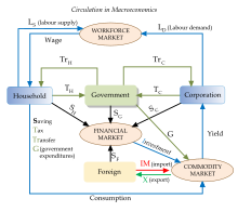
Macroeconomics takes a big-picture view of the entire economy, including examining the roles of, and relationships between, firms, households and governments, and the different types of markets, such as the financial market and the labour market

Macroeconomics is a branch of economics that deals with the performance, structure, behavior, and decision-making of an economy as a whole. This includes regional, national, and global economies. Macroeconomists study topics such as output/GDP (Gross Domestic Product) and national income, unemployment (including unemployment rates), price indices and inflation, consumption, saving, investment, energy, international trade, and international finance.

Macroeconomics and microeconomics are the two most general fields in economics. The focus of macroeconomics is often on a country (or larger entities like the whole world) and how its markets interact to produce large-scale phenomena that economists refer to as aggregate variables. In microeconomics the focus of analysis is often a single market, such as whether changes in supply or demand are to blame for price increases in the oil and automotive sectors. From introductory classes in "principles of economics" through doctoral studies, the macro/micro divide is institutionalized in the field of economics. Most economists identify as either macro- or micro-economists.

Macroeconomics is traditionally divided into topics along different time frames: the analysis of short-term fluctuations over the business cycle, the determination of structural levels of variables like inflation and unemployment in the medium (i.e. unaffected by short-term deviations) term, and the study of long-term economic growth. It also studies the consequences of policies targeted at mitigating fluctuations like fiscal or monetary policy, using taxation and government expenditure or interest rates, respectively, and of policies that can affect living standards in the long term, e.g. by affecting growth rates.

Macroeconomics as a separate field of research and study is generally recognized to start in 1936, when John Maynard Keynes published his The General Theory of Employment, Interest and Money, but its intellectual predecessors are much older. Since World War II, various macroeconomic schools of thought like Keynesians, monetarists, new classical and new Keynesian economists have made contributions to the development of the macroeconomic research mainstream.

Basic macroeconomic concepts

Macroeconomics encompasses a variety of concepts and variables, but above all the three central macroeconomic variables are output, unemployment, and inflation. Besides, the time horizon varies for different types of macroeconomic topics, and this distinction is crucial for many research and policy debates. A further important dimension is that of an economy's openness, economic theory distinguishing sharply between closed economies and open economies.

Circulation in macroeconomics

Time frame

It is usual to distinguish between three time horizons in macroeconomics, each having its own focus on e.g. the determination of output:

  • the short run (e.g. a few years): Focus is on business cycle fluctuations and changes in aggregate demand which often drive them. Stabilization policies like monetary policy or fiscal policy are relevant in this time frame
  • the medium run (e.g. a decade): Over the medium run, the economy tends to an output level determined by supply factors like the capital stock, the technology level and the labor force, and unemployment tends to revert to its structural (or "natural") level. These factors move slowly, so that it is a reasonable approximation to take them as given in a medium-term time scale, though labour market policies and competition policy are instruments that may influence the economy's structures and hence also the medium-run equilibrium
  • the long run (e.g. a couple of decades or more): On this time scale, emphasis is on the determinants of long-run economic growth like accumulation of human and physical capital, technological innovations and demographic changes. Potential policies to influence these developments are education reforms, incentives to change saving rates or to increase R&D activities.

Output and income

National output is the total amount of everything a country produces in a given period of time. Everything that is produced and sold generates an equal amount of income. The total net output of the economy is usually measured as gross domestic product (GDP). Adding net factor incomes from abroad to GDP produces gross national income (GNI), which measures total income of all residents in the economy. In most countries, the difference between GDP and GNI are modest so that GDP can approximately be treated as total income of all the inhabitants as well, but in some countries, e.g. countries with very large net foreign assets (or debt), the difference may be considerable.

Economists interested in long-run increases in output study economic growth. Advances in technology, accumulation of machinery and other capital, and better education and human capital, are all factors that lead to increased economic output over time. However, output does not always increase consistently over time. Business cycles can cause short-term drops in output called recessions. Economists look for macroeconomic policies that prevent economies from slipping into either recessions or overheating and that lead to higher productivity levels and standards of living.

Unemployment

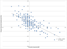
A chart using US data showing the relationship between economic growth and unemployment expressed by Okun's law. The relationship demonstrates cyclical unemployment. High short-run GDP growth leads to a lower unemployment rate.

The amount of unemployment in an economy is measured by the unemployment rate, i.e. the percentage of persons in the labor force who do not have a job, but who are actively looking for one. People who are retired, pursuing education, or discouraged from seeking work by a lack of job prospects are not part of the labor force and consequently not counted as unemployed, either.

Unemployment has a short-run cyclical component which depends on the business cycle, and a more permanent structural component, which can be loosely thought of as the average unemployment rate in an economy over extended periods, and which is often termed the natural or structural rate of unemployment.

Cyclical unemployment occurs when growth stagnates. Okun's law represents the empirical relationship between unemployment and short-run GDP growth. The original version of Okun's law states that a 3% increase in output would lead to a 1% decrease in unemployment.

The structural or natural rate of unemployment is the level of unemployment that will occur in a medium-run equilibrium, i.e. a situation with a cyclical unemployment rate of zero. There may be several reasons why there is some positive unemployment level even in a cyclically neutral situation, which all have their foundation in some kind of market failure:

  • Search unemployment (also called frictional unemployment) occurs when workers and firms are heterogeneous and there is imperfect information, generally causing a time-consuming search and matching process when filling a job vacancy in a firm, during which the prospective worker will often be unemployed. Sectoral shifts and other reasons for a changed demand from firms for workers with particular skills and characteristics, which occur continually in a changing economy, may also cause more search unemployment because of increased mismatch.
  • Efficiency wage models are labor market models in which firms choose not to lower wages to the level where supply equals demand because the lower wages would lower employees' efficiency levels.
  • Trade unions, which are important actors in the labor market in some countries, may exercise market power in order to keep wages over the market-clearing level for the benefice of their members even at the cost of some unemployment
  • Legal minimum wages may prevent the wage from falling to a market-clearing level, causing unemployment among low-skilled (and low-paid) workers. In the case of employers having some monopsony power, however, employment effects may have the opposite sign.

Inflation and deflation

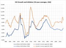
Changes in the ten-year moving averages of price level and growth in money supply (using the measure of M2, the supply of hard currency and money held in most types of bank accounts) in the US from 1880 to 2016. Over the long run, the two series show a clear positive correlation.

A general price increase across the entire economy is called inflation. When prices decrease, there is deflation. Economists measure these changes in prices with price indexes. Inflation will increase when an economy becomes overheated and grows too quickly. Similarly, a declining economy can lead to decreasing inflation and even in some cases deflation.

Central bankers conducting monetary policy usually have as a main priority to avoid too high inflation, typically by adjusting interest rates. High inflation as well as deflation can lead to increased uncertainty and other negative consequences, in particular when the inflation (or deflation) is unexpected. Consequently, most central banks aim for a positive, but stable and not very high inflation level.

Changes in the inflation level may be the result of several factors. Too much aggregate demand in the economy will cause an overheating, raising inflation rates via the Phillips curve because of a tight labor market leading to large wage increases which will be transmitted to increases in the price of the products of employers. Too little aggregate demand will have the opposite effect of creating more unemployment and lower wages, thereby decreasing inflation. Aggregate supply shocks will also affect inflation, e.g. the oil crises of the 1970s and the 2021–2023 global energy crisis. Changes in inflation may also impact the formation of inflation expectations, creating a self-fulfilling inflationary or deflationary spiral.

The monetarist quantity theory of money holds that changes in the price level are directly caused by changes in the money supply. Whereas there is empirical evidence that there is a long-run positive correlation between the growth rate of the money stock and the rate of inflation, the quantity theory has proved unreliable in the short- and medium-run time horizon relevant to monetary policy and is abandoned as a practical guideline by most central banks today.

Open economy macroeconomics

Open economy macroeconomics deals with the consequences of international trade in goods, financial assets and possibly factor markets like labor migration and international relocation of firms (physical capital). It explores what determines import, export, the balance of trade and over longer horizons the accumulation of net foreign assets. An important topic is the role of exchange rates and the pros and cons of maintaining a fixed exchange rate system or even a currency union like the Economic and Monetary Union of the European Union, drawing on the research literature on optimum currency areas.

Development

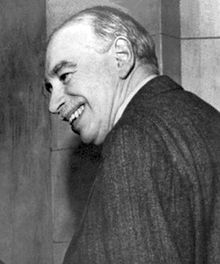
John Maynard Keynes is considered the initiator of macroeconomics when he published his work The General Theory of Employment, Interest, and Money in 1936

Macroeconomics as a separate field of research and study is generally recognized to start with the publication of John Maynard Keynes' The General Theory of Employment, Interest, and Money in 1936. The terms "macrodynamics" and "macroanalysis" were introduced by Ragnar Frisch in 1933, and Lawrence Klein in 1946 used the word "macroeconomics" itself in a journal title in 1946. but naturally several of the themes which are central to macroeconomic research had been discussed by thoughtful economists and other writers long before 1936.

Before Keynes

In particular, macroeconomic questions before Keynes were the topic of the two long-standing traditions of business cycle theory and monetary theory. William Stanley Jevons was one of the pioneers of the first tradition, whereas the quantity theory of money, labelled the oldest surviving theory in economics, as an example of the second was described already in the 16th century by Martín de Azpilcueta and later discussed by personalities like John Locke and David Hume. In the first decades of the 20th century monetary theory was dominated by the eminent economists Alfred Marshall, Knut Wicksell and Irving Fisher.

Keynes and Keynesian economics

When the Great Depression struck, the reigning economists had difficulty explaining how goods could go unsold and workers could be left unemployed. In the prevailing neoclassical economics paradigm, prices and wages would drop until the market cleared, and all goods and labor were sold. Keynes in his main work, the General Theory, initiated what is known as the Keynesian revolution. He offered a new interpretation of events and a whole intellectural framework - a novel theory of economics that explained why markets might not clear, which would evolve into a school of thought known as Keynesian economics, also called Keynesianism or Keynesian theory.

In Keynes' theory, aggregate demand - by Keynes called "effective demand" - was key to determining output. Even if Keynes conceded that output might eventually return to a medium-run equilibrium (or "potential") level, the process would be slow at best. Keynes coined the term liquidity preference (his preferred name for what is also known as money demand) and explained how monetary policy might affect aggregate demand, at the same time offering clear policy recommendations for an active role of fiscal policy in stabilizing aggregate demand and hence output and employment. In addition, he explained how the multiplier effect would magnify a small decrease in consumption or investment and cause declines throughout the economy, and noted the role that uncertainty and animal spirits can play in the economy.

The generation following Keynes combined the macroeconomics of the General Theory with neoclassical microeconomics to create the neoclassical synthesis. By the 1950s, most economists had accepted the synthesis view of the macroeconomy. Economists like Paul Samuelson, Franco Modigliani, James Tobin, and Robert Solow developed formal Keynesian models and contributed formal theories of consumption, investment, and money demand that fleshed out the Keynesian framework.

Monetarism

Milton Friedman updated the quantity theory of money to include a role for money demand. He argued that the role of money in the economy was sufficient to explain the Great Depression, and that aggregate demand oriented explanations were not necessary. Friedman also argued that monetary policy was more effective than fiscal policy; however, Friedman doubted the government's ability to "fine-tune" the economy with monetary policy. He generally favored a policy of steady growth in money supply instead of frequent intervention.

Friedman also challenged the original simple Phillips curve relationship between inflation and unemployment. Friedman and Edmund Phelps (who was not a monetarist) proposed an "augmented" version of the Phillips curve that excluded the possibility of a stable, long-run tradeoff between inflation and unemployment. When the oil shocks of the 1970s created a high unemployment and high inflation, Friedman and Phelps were vindicated. Monetarism was particularly influential in the early 1980s, but fell out of favor when central banks found the results disappointing when trying to target money supply instead of interest rates as monetarists recommended, concluding that the relationships between money growth, inflation and real GDP growth are too unstable to be useful in practical monetary policy making.

New classical economics

New classical macroeconomics further challenged the Keynesian school. A central development in new classical thought came when Robert Lucas introduced rational expectations to macroeconomics. Prior to Lucas, economists had generally used adaptive expectations where agents were assumed to look at the recent past to make expectations about the future. Under rational expectations, agents are assumed to be more sophisticated. Consumers will not simply assume a 2% inflation rate just because that has been the average the past few years; they will look at current monetary policy and economic conditions to make an informed forecast. In the new classical models with rational expectations, monetary policy only had a limited impact.

Lucas also made an influential critique of Keynesian empirical models. He argued that forecasting models based on empirical relationships would keep producing the same predictions even as the underlying model generating the data changed. He advocated models based on fundamental economic theory (i.e. having an explicit microeconomic foundation) that would, in principle, be structurally accurate as economies changed.

Following Lucas's critique, new classical economists, led by Edward C. Prescott and Finn E. Kydland, created real business cycle (RBC) models of the macro economy. RBC models were created by combining fundamental equations from neo-classical microeconomics to make quantitative models. In order to generate macroeconomic fluctuations, RBC models explained recessions and unemployment with changes in technology instead of changes in the markets for goods or money. Critics of RBC models argue that technological changes, which typically diffuse slowly throughout the economy, could hardly generate the large short-run output fluctuations that we observe. In addition, there is strong empirical evidence that monetary policy does affect real economic activity, and the idea that technological regress can explain recent recessions seems implausible.

Despite criticism of the realism in the RBC models, they have been very influential in economic methodology by providing the first examples of general equilibrium models based on microeconomic foundations and a specification of underlying shocks that aim to explain the main features of macroeconomic fluctuations, not only qualitatively, but also quantitatively. In this way, they were forerunners of the later DSGE models.

New Keynesian response

New Keynesian economists responded to the new classical school by adopting rational expectations and focusing on developing micro-founded models that were immune to the Lucas critique. Like classical models, new classical models had assumed that prices would be able to adjust perfectly and monetary policy would only lead to price changes. New Keynesian models investigated sources of sticky prices and wages due to imperfect competition, which would not adjust, allowing monetary policy to impact quantities instead of prices. Stanley Fischer and John B. Taylor produced early work in this area by showing that monetary policy could be effective even in models with rational expectations when contracts locked in wages for workers. Other new Keynesian economists, including Olivier Blanchard, Janet Yellen, Julio Rotemberg, Greg Mankiw, David Romer, and Michael Woodford, expanded on this work and demonstrated other cases where various market imperfections caused inflexible prices and wages leading in turn to monetary and fiscal policy having real effects. Other researchers focused on imperferctions in labor markets, developing models of efficiency wages or search and matching (SAM) models, or imperfections in credit markets like Ben Bernanke.

By the late 1990s, economists had reached a rough consensus. The market imperfections and nominal rigidities of new Keynesian theory was combined with rational expectations and the RBC methodology to produce a new and popular type of models called dynamic stochastic general equilibrium (DSGE) models. The fusion of elements from different schools of thought has been dubbed the new neoclassical synthesis. These models are now used by many central banks and are a core part of contemporary macroeconomics.

After the global financial crisis

The global financial crisis leading to the Great Recession led to major reassessment of macroeconomics, which as a field generally had neglected the potential role of financial institutions in the economy. After the crisis, macroeconomic researchers have turned their attention in several new directions:

  • the financial system and the nature of macrofinancial linkages and frictions, studying leverage, liquidity and complexity problems in the financial sector, the use of macroprudential tools and the dangers of an unsustainable public debt
  • increased emphasis on empirical work as part of the so-called credibility revolution in economics, using improved methods to distinguish between correlation and causality to improve future policy discussions
  • interest in understanding the importance of heterogeneity among the economic agents, leading among other examples to the construction of heterogeneous agent new Keynesian models (HANK models), which may potentially also improve understanding of the impact of macroeconomics on the income distribution
  • understanding the implications of integrating the findings of the increasingly useful behavioral economics literature into macroeconomics and behavioral finance

Growth models

Research in the economics of the determinants behind long-run economic growth has followed its own course. The Harrod-Domar model from the 1940s attempted to build a long-run growth model inspired by Keynesian demand-driven considerations. The Solow–Swan model worked out by Robert Solow and, independently, Trevor Swan in the 1950s achieved more long-lasting success, however, and is still today a common textbook model for explaining economic growth in the long-run. The model operates with a production function where national output is the product of two inputs: capital and labor. The Solow model assumes that labor and capital are used at constant rates without the fluctuations in unemployment and capital utilization commonly seen in business cycles. In this model, increases in output, i.e. economic growth, can only occur because of an increase in the capital stock, a larger population, or technological advancements that lead to higher productivity (total factor productivity). An increase in the savings rate leads to a temporary increase as the economy creates more capital, which adds to output. However, eventually the depreciation rate will limit the expansion of capital: savings will be used up replacing depreciated capital, and no savings will remain to pay for an additional expansion in capital. Solow's model suggests that economic growth in terms of output per capita depends solely on technological advances that enhance productivity. The Solow model can be interpreted as a special case of the more general Ramsey growth model, where households' savings rates are not constant as in the Solow model, but derived from an explicit intertemporal utility function.

In the 1980s and 1990s endogenous growth theory arose to challenge the neoclassical growth theory of Ramsey and Solow. This group of models explains economic growth through factors such as increasing returns to scale for capital and learning-by-doing that are endogenously determined instead of the exogenous technological improvement used to explain growth in Solow's model. Another type of endogenous growth models endogenized the process of technological progress by modelling research and development activities by profit-maximizing firms explicitly within the growth models themselves.

Environmental and climate issues

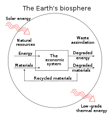
Natural resources flow through the economy and end up as waste and pollution.

Since the 1970s, various environmental problems have been integrated into growth and other macroeconomic models to study their implications more thoroughly. During the oil crises of the 1970s when scarcity problems of natural resources were high on the public agenda, economists like Joseph Stiglitz and Robert Solow introduced non-renewable resources into neoclassical growth models to study the possibilities of maintaining growth in living standards under these conditions. More recently, the issue of climate change and the possibilities of a sustainable development are examined in so-called integrated assessment models, pioneered by William Nordhaus. In macroeconomic models in environmental economics, the economic system is dependant upon the environment. In this case, the circular flow of income diagram may be replaced by a more complex flow diagram reflecting the input of solar energy, which sustains natural inputs and environmental services which are then used as units of production. Once consumed, natural inputs pass out of the economy as pollution and waste. The potential of an environment to provide services and materials is referred to as an "environment's source function", and this function is depleted as resources are consumed or pollution contaminates the resources. The "sink function" describes an environment's ability to absorb and render harmless waste and pollution: when waste output exceeds the limit of the sink function, long-term damage occurs.

Macroeconomic policy

The division into various time frames of macroeconomic research leads to a parallel division of macroeconomic policies into short-run policies aimed at mitigating the harmful consequences of business cycles (known as stabilization policy) and medium- and long-run policies targeted at improving the structural levels of macroeconomic variables.

Stabilization policy is usually implemented through two sets of tools: fiscal and monetary policy. Both forms of policy are used to stabilize the economy, i.e. limiting the effects of the business cycle by conducting expansive policy when the economy is in a recession or contractive policy in the case of overheating.

Structural policies may be labor market policies which aim to change the structural unemployment rate or policies which affect long-run propensities to save, invest, or engage in education or research and development.

Monetary policy

Central banks conduct monetary policy mainly by adjusting short-term interest rates.[39] The actual method through which the interest rate is changed differs from central bank to central bank, but typically the implementation happens either directly via administratively changing the central bank's own offered interest rates or indirectly via open market operations.

Via the monetary transmission mechanism, interest rate changes affect investment, consumption, asset prices like stock prices and house prices, and through exchange rate reactions export and import. In this way aggregate demand, employment and ultimately inflation is affected. Expansionary monetary policy lowers interest rates, increasing economic activity, whereas contractionary monetary policy raises interest rates. In the case of a fixed exchange rate system, interest rate decisions together with direct intervention in the foreign exchange market are major tools to control the exchange rate.

In developed countries, most central banks follow inflation targeting, focusing on keeping medium-term inflation close to an explicit target, say 2%, or within an explicit range. This includes the Federal Reserve and the European Central Bank, which are generally considered to follow a strategy very close to inflation targeting, even though they do not officially label themselves as inflation targeters. In practice, an official inflation targeting often leaves room for the central bank to also help stabilize output and employment, a strategy known as "flexible inflation targeting". Most emerging economies focus their monetary policy on maintaining a fixed exchange rate regime, aligning their currency with one or more foreign currencies, typically the US dollar or the euro.

Conventional monetary policy can be ineffective in situations such as a liquidity trap. When nominal interest rates are near zero, central banks cannot loosen monetary policy through conventional means. In that situation, they may use unconventional monetary policy such as quantitative easing to help stabilize output. Quantity easing can be implemented by buying not only government bonds, but also other assets such as corporate bonds, stocks, and other securities. This allows lower interest rates for a broader class of assets beyond government bonds. A similar strategy is to lower long-term interest rates by buying long-term bonds and selling short-term bonds to create a flat yield curve, known in the US as Operation Twist.

Fiscal policy

Fiscal policy is the use of government's revenue (taxes) and expenditure as instruments to influence the economy.

For example, if the economy is producing less than potential output, government spending can be used to employ idle resources and boost output, or taxes could be lowered to boost private consumption which has a similar effect. Government spending or tax cuts do not have to make up for the entire output gap. There is a multiplier effect that affects the impact of government spending. For instance, when the government pays for a bridge, the project not only adds the value of the bridge to output, but also allows the bridge workers to increase their consumption and investment, which helps to close the output gap.

The effects of fiscal policy can be limited by partial or full crowding out. When the government takes on spending projects, it limits the amount of resources available for the private sector to use. Full crowding out occurs in the extreme case when government spending simply replaces private sector output instead of adding additional output to the economy. A crowding out effect may also occur if government spending should lead to higher interest rates, which would limit investment.

Some fiscal policy is implemented through automatic stabilizers without any active decisions by politicians. Automatic stabilizers do not suffer from the policy lags of discretionary fiscal policy. Automatic stabilizers use conventional fiscal mechanisms, but take effect as soon as the economy takes a downturn: spending on unemployment benefits automatically increases when unemployment rises, and tax revenues decrease, which shelters private income and consumption from part of the fall in market income.

Comparison of fiscal and monetary policy

There is a general consensus that both monetary and fiscal instruments may affect demand and activity in the short run (i.e. over the business cycle). Economists usually favor monetary over fiscal policy to mitigate moderate fluctuations, however, because it has two major advantages. First, monetary policy is generally implemented by independent central banks instead of the political institutions that control fiscal policy. Independent central banks are less likely to be subject to political pressures for overly expansionary policies. Second, monetary policy may suffer shorter inside lags and outside lags than fiscal policy. There are some exceptions, however: Firstly, in the case of a major shock, monetary stabilization policy may not be sufficient and should be supplemented by active fiscal stabilization. Secondly, in the case of a very low interest level, the economy may be in a liquidity trap in which monetary policy becomes ineffective, which makes fiscal policy the more potent tool to stabilize the economy. Thirdly, in regimes where monetary policy is tied to fulfilling other targets, in particular fixed exchange rate regimes, the central bank cannot simultaneously adjust its interest rates to mitigate domestic business cycle fluctuations, making fiscal policy the only usable tool for such countries.

Macroeconomic models

Macroeconomic teaching, research and informed debates normally evolve around formal (diagrammatic or equational) macroeconomic models to clarify assumptions and show their consequences in a precise way. Models include simple theoretical models, often containing only a few equations, used in teaching and research to highlight key basic principles, and larger applied quantitative models used by e.g. governments, central banks, think tanks and international organisations to predict effects of changes in economic policy or other exogenous factors or as a basis for making economic forecasting.

Well-known specific theoretical models include short-term models like the Keynesian cross, the IS–LM model and the Mundell–Fleming model, medium-term models like the AD–AS model, building upon a Phillips curve, and long-term growth models like the Solow–Swan model, the Ramsey–Cass–Koopmans model and Peter Diamond's overlapping generations model. Quantitative models include early large-scale macroeconometric model, the new classical real business cycle models, microfounded computable general equilibrium (CGE) models used for medium-term (structural) questions like international trade or tax reforms, Dynamic stochastic general equilibrium (DSGE) models used to analyze business cycles, not least in many central banks, or integrated assessment models like DICE.

Specific models

IS–LM model

In this example of a traditional IS–LM chart, the IS curve moves to the right, causing higher interest rates (i) and expansion in the "real" economy (real GDP, or Y).

The IS–LM model, invented by John Hicks in 1936, gives the underpinnings of aggregate demand (itself discussed below). It answers the question "At any given price level, what is the quantity of goods demanded?" The graphic model shows combinations of interest rates and output that ensure equilibrium in both the goods and money markets under the model's assumptions. The goods market is modeled as giving equality between investment and public and private saving (IS), and the money market is modeled as giving equilibrium between the money supply and liquidity preference (equivalent to money demand).

The IS curve consists of the points (combinations of income and interest rate) where investment, given the interest rate, is equal to public and private saving, given output. The IS curve is downward sloping because output and the interest rate have an inverse relationship in the goods market: as output increases, more income is saved, which means interest rates must be lower to spur enough investment to match saving.

The traditional LM curve is upward sloping because the interest rate and output have a positive relationship in the money market: as income (identically equal to output in a closed economy) increases, the demand for money increases, resulting in a rise in the interest rate in order to just offset the incipient rise in money demand.

The IS-LM model is often used in elementary textbooks to demonstrate the effects of monetary and fiscal policy, though it ignores many complexities of most modern macroeconomic models. A problem related to the LM curve is that modern central banks largely ignore the money supply in determining policy, contrary to the model's basic assumptions. In some modern textbooks, consequently, the traditional IS-LM model has been modified by replacing the traditional LM curve with an assumption that the central bank simply determines the interest rate of the economy directly.

AD-AS model

A traditional AD–AS diagram showing a shift in AD, and the AS curve becoming inelastic beyond potential output

The AD–AS model is a common textbook model for explaining the macroeconomy. The original version of the model shows the price level and level of real output given the equilibrium in aggregate demand and aggregate supply. The aggregate demand curve's downward slope means that more output is demanded at lower price levels. The downward slope can be explained as the result of three effects: the Pigou or real balance effect, which states that as real prices fall, real wealth increases, resulting in higher consumer demand of goods; the Keynes or interest rate effect, which states that as prices fall, the demand for money decreases, causing interest rates to decline and borrowing for investment and consumption to increase; and the net export effect, which states that as prices rise, domestic goods become comparatively more expensive to foreign consumers, leading to a decline in exports.

In many representations of the AD–AS model, the aggregate supply curve is horizontal at low levels of output and becomes inelastic near the point of potential output, which corresponds with full employment. Since the economy cannot produce beyond the potential output, any AD expansion will lead to higher price levels instead of higher output.

In modern textbooks, the AD–AS model is often presented sligthly differently, however, in a diagram showing not the price level, but the inflation rate along the vertical axis, making it easier to relate the diagram to real-world policy discussions. In this framework, the AD curve is downward sloping because higher inflation will cause the central bank, which is assumed to follow an inflation target, to raise the interest rate which will dampen economic activity, hence reducing output. The AS curve is upward sloping following a standard modern Phillips curve thought, in which a higher level of economic activity lowers unemployment, leading to higher wage growth and in turn higher inflation.

Lie point symmetry

From Wikipedia, the free encyclopedia https://en.wikipedia.org/wiki/Lie_point_symmetry     ...