Feature (computer vision)

From Wikipedia, the free encyclopedia

https://en.wikipedia.org/wiki/Feature_(computer_vision) 

 

See also: Feature (machine learning)

In computer vision and image processing, a feature is a piece of information about the content of an image; typically about whether a certain region of the image has certain properties. Features may be specific structures in the image such as points, edges or objects. Features may also be the result of a general neighborhood operation or feature detection applied to the image. Other examples of features are related to motion in image sequences, or to shapes defined in terms of curves or boundaries between different image regions.

More broadly a feature is any piece of information which is relevant for solving the computational task related to a certain application. This is the same sense as feature in machine learning and pattern recognition generally, though image processing has a very sophisticated collection of features. The feature concept is very general and the choice of features in a particular computer vision system may be highly dependent on the specific problem at hand.

Definition

There is no universal or exact definition of what constitutes a feature, and the exact definition often depends on the problem or the type of application. Nevertheless, a feature is typically defined as an "interesting" part of an image, and features are used as a starting point for many computer vision algorithms.

Since features are used as the starting point and main primitives for subsequent algorithms, the overall algorithm will often only be as good as its feature detector. Consequently, the desirable property for a feature detector is repeatability: whether or not the same feature will be detected in two or more different images of the same scene.

Feature detection is a low-level image processing operation. That is, it is usually performed as the first operation on an image, and examines every pixel to see if there is a feature present at that pixel. If this is part of a larger algorithm, then the algorithm will typically only examine the image in the region of the features. As a built-in pre-requisite to feature detection, the input image is usually smoothed by a Gaussian kernel in a scale-space representation and one or several feature images are computed, often expressed in terms of local image derivative operations.

Occasionally, when feature detection is computationally expensive and there are time constraints, a higher level algorithm may be used to guide the feature detection stage, so that only certain parts of the image are searched for features.

There are many computer vision algorithms that use feature detection as the initial step, so as a result, a very large number of feature detectors have been developed. These vary widely in the kinds of feature detected, the computational complexity and the repeatability.

When features are defined in terms of local neighborhood operations applied to an image, a procedure commonly referred to as feature extraction, one can distinguish between feature detection approaches that produce local decisions whether there is a feature of a given type at a given image point or not, and those who produce non-binary data as result. The distinction becomes relevant when the resulting detected features are relatively sparse. Although local decisions are made, the output from a feature detection step does not need to be a binary image. The result is often represented in terms of sets of (connected or unconnected) coordinates of the image points where features have been detected, sometimes with subpixel accuracy.

When feature extraction is done without local decision making, the result is often referred to as a feature image. Consequently, a feature image can be seen as an image in the sense that it is a function of the same spatial (or temporal) variables as the original image, but where the pixel values hold information about image features instead of intensity or color. This means that a feature image can be processed in a similar way as an ordinary image generated by an image sensor. Feature images are also often computed as integrated step in algorithms for feature detection.

Feature vectors and feature spaces

In some applications, it is not sufficient to extract only one type of feature to obtain the relevant information from the image data. Instead two or more different features are extracted, resulting in two or more feature descriptors at each image point. A common practice is to organize the information provided by all these descriptors as the elements of one single vector, commonly referred to as a feature vector. The set of all possible feature vectors constitutes a feature space.

A common example of feature vectors appears when each image point is to be classified as belonging to a specific class. Assuming that each image point has a corresponding feature vector based on a suitable set of features, meaning that each class is well separated in the corresponding feature space, the classification of each image point can be done using standard classification method.

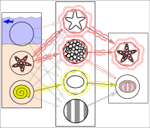
Simplified example of training a neural network in object detection: The network is trained by multiple images that are known to depict starfish and sea urchins, which are correlated with "nodes" that represent visual features. The starfish match with a ringed texture and a star outline, whereas most sea urchins match with a striped texture and oval shape. However, the instance of a ring textured sea urchin creates a weakly weighted association between them.

 

Subsequent run of the network on an input image (left): The network correctly detects the starfish. However, the weakly weighted association between ringed texture and sea urchin also confers a weak signal to the latter from one of two features. In addition, a shell that was not included in the training gives a weak signal for the oval shape, also resulting in a weak signal for the sea urchin output. These weak signals may result in a false positive result for sea urchin.
In reality, textures and outlines would not be represented by single nodes, but rather by associated weight patterns of multiple nodes.

Another and related example occurs when neural network-based processing is applied to images. The input data fed to the neural network is often given in terms of a feature vector from each image point, where the vector is constructed from several different features extracted from the image data. During a learning phase, the network can itself find which combinations of different features are useful for solving the problem at hand.

Types

Edges

Edges are points where there is a boundary (or an edge) between two image regions. In general, an edge can be of almost arbitrary shape, and may include junctions. In practice, edges are usually defined as sets of points in the image which have a strong gradient magnitude. Furthermore, some common algorithms will then chain high gradient points together to form a more complete description of an edge. These algorithms usually place some constraints on the properties of an edge, such as shape, smoothness, and gradient value.

Locally, edges have a one-dimensional structure.

Corners / interest points

The terms corners and interest points are used somewhat interchangeably and refer to point-like features in an image, which have a local two dimensional structure. The name "Corner" arose since early algorithms first performed edge detection, and then analysed the edges to find rapid changes in direction (corners). These algorithms were then developed so that explicit edge detection was no longer required, for instance by looking for high levels of curvature in the image gradient. It was then noticed that the so-called corners were also being detected on parts of the image which were not corners in the traditional sense (for instance a small bright spot on a dark background may be detected). These points are frequently known as interest points, but the term "corner" is used by tradition.

Blobs / regions of interest points

Blobs provide a complementary description of image structures in terms of regions, as opposed to corners that are more point-like. Nevertheless, blob descriptors may often contain a preferred point (a local maximum of an operator response or a center of gravity) which means that many blob detectors may also be regarded as interest point operators. Blob detectors can detect areas in an image which are too smooth to be detected by a corner detector.

Consider shrinking an image and then performing corner detection. The detector will respond to points which are sharp in the shrunk image, but may be smooth in the original image. It is at this point that the difference between a corner detector and a blob detector becomes somewhat vague. To a large extent, this distinction can be remedied by including an appropriate notion of scale. Nevertheless, due to their response properties to different types of image structures at different scales, the LoG and DoH blob detectors are also mentioned in the article on corner detection.

Ridges

For elongated objects, the notion of ridges is a natural tool. A ridge descriptor computed from a grey-level image can be seen as a generalization of a medial axis. From a practical viewpoint, a ridge can be thought of as a one-dimensional curve that represents an axis of symmetry, and in addition has an attribute of local ridge width associated with each ridge point. Unfortunately, however, it is algorithmically harder to extract ridge features from general classes of grey-level images than edge-, corner- or blob features. Nevertheless, ridge descriptors are frequently used for road extraction in aerial images and for extracting blood vessels in medical images—see ridge detection.

Detection

Feature detection includes methods for computing abstractions of image information and making local decisions at every image point whether there is an image feature of a given type at that point or not. The resulting features will be subsets of the image domain, often in the form of isolated points, continuous curves or connected regions.

The extraction of features are sometimes made over several scalings. One of these methods is the scale-invariant feature transform (SIFT).

Further information on Combination Of Shifted FIlter REsponses: COSFIRE

Common feature detectors and their classification:

Feature detector	Edge	Corner	Blob	Ridge
Canny	Yes	No	No	No
Sobel	Yes	No	No	No
Harris & Stephens / Plessey	Yes	Yes	No	No
SUSAN	Yes	Yes	No	No
Shi & Tomasi	No	Yes	No	No
Level curve curvature	No	Yes	No	No
FAST	No	Yes	Yes	No
Laplacian of Gaussian	No	Yes	Yes	No
Difference of Gaussians	No	Yes	Yes	No
Determinant of Hessian	No	Yes	Yes	No
Hessian strength feature measures	No	Yes	Yes	No
MSER	No	No	Yes	No
Principal curvature ridges	No	No	No	Yes
Grey-level blobs	No	No	Yes	No

Extraction

For broader coverage of this topic, see Feature extraction (machine learning).

Once features have been detected, a local image patch around the feature can be extracted. This extraction may involve quite considerable amounts of image processing. The result is known as a feature descriptor or feature vector. Among the approaches that are used to feature description, one can mention N-jets and local histograms (see scale-invariant feature transform for one example of a local histogram descriptor). In addition to such attribute information, the feature detection step by itself may also provide complementary attributes, such as the edge orientation and gradient magnitude in edge detection and the polarity and the strength of the blob in blob detection.

Low-level

• Edge detection
• Corner detection
• Blob detection
• Ridge detection
• Scale-invariant feature transform

Curvature

• Edge direction, changing intensity, autocorrelation.

Image motion

• Motion detection. Area based, differential approach. Optical flow.

Shape based

• Thresholding
• Blob extraction
• Template matching
• Hough transform
  • Lines
  • Circles/ellipses
  • Arbitrary shapes (generalized Hough transform)
  • Works with any parameterizable feature (class variables, cluster detection, etc..)
• Generalised Hough transform

Flexible methods

• Deformable, parameterized shapes
• Active contours (snakes)

Representation

Main article: Visual descriptor

A specific image feature, defined in terms of a specific structure in the image data, can often be represented in different ways. For example, an edge can be represented as a boolean variable in each image point that describes whether an edge is present at that point. Alternatively, we can instead use a representation which provides a certainty measure instead of a boolean statement of the edge's existence and combine this with information about the orientation of the edge. Similarly, the color of a specific region can either be represented in terms of the average color (three scalars) or a color histogram (three functions).

When a computer vision system or computer vision algorithm is designed the choice of feature representation can be a critical issue. In some cases, a higher level of detail in the description of a feature may be necessary for solving the problem, but this comes at the cost of having to deal with more data and more demanding processing. Below, some of the factors which are relevant for choosing a suitable representation are discussed. In this discussion, an instance of a feature representation is referred to as a feature descriptor, or simply descriptor.

Certainty or confidence

Two examples of image features are local edge orientation and local velocity in an image sequence. In the case of orientation, the value of this feature may be more or less undefined if more than one edge are present in the corresponding neighborhood. Local velocity is undefined if the corresponding image region does not contain any spatial variation. As a consequence of this observation, it may be relevant to use a feature representation which includes a measure of certainty or confidence related to the statement about the feature value. Otherwise, it is a typical situation that the same descriptor is used to represent feature values of low certainty and feature values close to zero, with a resulting ambiguity in the interpretation of this descriptor. Depending on the application, such an ambiguity may or may not be acceptable.

In particular, if a featured image will be used in subsequent processing, it may be a good idea to employ a feature representation that includes information about certainty or confidence. This enables a new feature descriptor to be computed from several descriptors, for example computed at the same image point but at different scales, or from different but neighboring points, in terms of a weighted average where the weights are derived from the corresponding certainties. In the simplest case, the corresponding computation can be implemented as a low-pass filtering of the featured image. The resulting feature image will, in general, be more stable to noise.

Averageability

In addition to having certainty measures included in the representation, the representation of the corresponding feature values may itself be suitable for an averaging operation or not. Most feature representations can be averaged in practice, but only in certain cases can the resulting descriptor be given a correct interpretation in terms of a feature value. Such representations are referred to as averageable.

For example, if the orientation of an edge is represented in terms of an angle, this representation must have a discontinuity where the angle wraps from its maximal value to its minimal value. Consequently, it can happen that two similar orientations are represented by angles which have a mean that does not lie close to either of the original angles and, hence, this representation is not averageable. There are other representations of edge orientation, such as the structure tensor, which are averageable.

Another example relates to motion, where in some cases only the normal velocity relative to some edge can be extracted. If two such features have been extracted and they can be assumed to refer to same true velocity, this velocity is not given as the average of the normal velocity vectors. Hence, normal velocity vectors are not averageable. Instead, there are other representations of motions, using matrices or tensors, that give the true velocity in terms of an average operation of the normal velocity descriptors.

Matching

Main article: Correspondence problem

Features detected in each image can be matched across multiple images to establish corresponding features such as corresponding points.

The algorithm is based on comparing and analyzing point correspondences between the reference image and the target image. If any part of the cluttered scene shares correspondences greater than the threshold, that part of the cluttered scene image is targeted and considered to include the reference object there.

Agricultural robot

From Wikipedia, the free encyclopedia

https://en.wikipedia.org/wiki/Agricultural_robot 

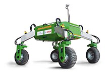
Autonomous agricultural robot

An agricultural robot is a robot deployed for agricultural purposes. The main area of application of robots in agriculture today is at the harvesting stage. Emerging applications of robots or drones in agriculture include weed control, cloud seeding, planting seeds, harvesting, environmental monitoring and soil analysis.According to Verified Market Research, the agricultural robots market is expected to reach $11.58 billion by 2025.

General

Fruit picking robots, driverless tractor / sprayers, and sheep shearing robots are designed to replace human labor. In most cases, a lot of factors have to be considered (e.g., the size and color of the fruit to be picked) before the commencement of a task. Robots can be used for other horticultural tasks such as pruning, weeding, spraying and monitoring. Robots can also be used in livestock applications (livestock robotics) such as automatic milking, washing and castrating. Robots like these have many benefits for the agricultural industry, including a higher quality of fresh produce, lower production costs, and a decreased need for manual labor. They can also be used to automate manual tasks, such as weed or bracken spraying, where the use of tractors and other human-operated vehicles is too dangerous for the operators.

Designs

Fieldwork robot

The mechanical design consists of an end effector, manipulator, and gripper. Several factors must be considered in the design of the manipulator, including the task, economic efficiency, and required motions. The end effector influences the market value of the fruit and the gripper's design is based on the crop that is being harvested.

End effector

An end effector in an agricultural robot is the device found at the end of the robotic arm, used for various agricultural operations. Several different kinds of end effectors have been developed. In an agricultural operation involving grapes in Japan, end effectors are used for harvesting, berry-thinning, spraying, and bagging. Each was designed according to the nature of the task and the shape and size of the target fruit. For instance, the end effectors used for harvesting were designed to grasp, cut, and push the bunches of grapes.

Berry thinning is another operation performed on the grapes, and is used to enhance the market value of the grapes, increase the grapes' size, and facilitate the bunching process. For berry thinning, an end effector consists of an upper, middle, and lower part. The upper part has two plates and a rubber that can open and close. The two plates compress the grapes to cut off the rachis branches and extract the bunch of grapes. The middle part contains a plate of needles, a compression spring, and another plate which has holes spread across its surface. When the two plates compress, the needles punch holes through the grapes. Next, the lower part has a cutting device which can cut the bunch to standardize its length.

For spraying, the end effector consists of a spray nozzle that is attached to a manipulator. In practice, producers want to ensure that the chemical liquid is evenly distributed across the bunch. Thus, the design allows for an even distribution of the chemical by making the nozzle move at a constant speed while keeping distance from the target.

The final step in grape production is the bagging process. The bagging end effector is designed with a bag feeder and two mechanical fingers. In the bagging process, the bag feeder is composed of slits which continuously supply bags to the fingers in an up and down motion. While the bag is being fed to the fingers, two leaf springs that are located on the upper end of the bag hold the bag open. The bags are produced to contain the grapes in bunches. Once the bagging process is complete, the fingers open and release the bag. This shuts the leaf springs, which seal the bag and prevent it from opening again.

Gripper

The gripper is a grasping device that is used for harvesting the target crop. Design of the gripper is based on simplicity, low cost, and effectiveness. Thus, the design usually consists of two mechanical fingers that are able to move in synchrony when performing their task. Specifics of the design depend on the task that is being performed. For example, in a procedure that required plants to be cut for harvesting, the gripper was equipped with a sharp blade.

Manipulator

The manipulator allows the gripper and end effector to navigate through their environment. The manipulator consists of four-bar parallel links that maintain the gripper's position and height. The manipulator also can utilize one, two, or three pneumatic actuators. Pneumatic actuators are motors which produce linear and rotary motion by converting compressed air into energy. The pneumatic actuator is the most effective actuator for agricultural robots because of its high power-weight ratio. The most cost efficient design for the manipulator is the single actuator configuration, yet this is the least flexible option.

Development

The first development of robotics in agriculture can be dated as early as the 1920s, with research to incorporate automatic vehicle guidance into agriculture beginning to take shape. This research led to the advancements between the 1950s and 60s of autonomous agricultural vehicles. The concept was not perfect however, with the vehicles still needing a cable system to guide their path. Robots in agriculture continued to develop as technologies in other sectors began to develop as well. It was not until the 1980s, following the development of the computer, that machine vision guidance became possible.

Other developments over the years included the harvesting of oranges using a robot both in France and the US.

While robots have been incorporated in indoor industrial settings for decades, outdoor robots for the use of agriculture are considered more complex and difficult to develop. This is due to concerns over safety, but also over the complexity of picking crops subject to different environmental factors and unpredictability.

Demand in the market

There are concerns over the amount of labor the agricultural sector needs. With an aging population, Japan is unable to meet the demands of the agricultural labor market. Similarly, the United States currently depends on a large number of immigrant workers, but between the decrease in seasonal farmworkers and increased efforts to stop immigration by the government, they too are unable to meet the demand. Businesses are often forced to let crops rot due to an inability to pick them all by the end of the season. Additionally, there are concerns over the growing population that will need to be fed over the next years. Because of this, there is a large desire to improve agricultural machinery to make it more cost efficient and viable for continued use.

Current applications and trends

Unmanned tractor "Uralets-224"

Much of the current research continues to work towards autonomous agricultural vehicles. This research is based on the advancements made in driver-assist systems and self-driving cars.

While robots have already been incorporated in many areas of agricultural farm work, they are still largely missing in the harvest of various crops. This has started to change as companies begin to develop robots that complete more specific tasks on the farm. The biggest concern over robots harvesting crops comes from harvesting soft crops such as strawberries which can easily be damaged or missed entirely. Despite these concerns, progress in this area is being made. According to Gary Wishnatzki, the co-founder of Harvest Croo Robotics, one of their strawberry pickers currently being tested in Florida can "pick a 25-acre field in just three days and replace a crew of about 30 farm workers". Similar progress is being made in harvesting apples, grapes, and other crops. In the case of apple harvesting robots, current developments have been too slow to be commercially viable. Modern robots are able to harvest apples at a rate of one every five to ten seconds while the average human harvests at a rate of one per second.

Another goal being set by agricultural companies involves the collection of data. There are rising concerns over the growing population and the decreasing labor available to feed them. Data collection is being developed as a way to increase productivity on farms. AgriData is currently developing new technology to do just this and help farmers better determine the best time to harvest their crops by scanning fruit trees.

Applications

See also: § General, and § Current applications and trends

Robots have many fields of application in agriculture. Some examples and prototypes of robots include the Merlin Robot Milker, Rosphere, Harvest Automation, Orange Harvester, lettuce bot, and weeder.

According to David Gardner, chief executive of the Royal Agricultural Society of England, a robot can complete a complicated task if its repetitive and the robot is allowed to sit in a single place. Furthermore, robots that work on repetitive tasks (e.g. milking) fulfill their role to a consistent and particular standard.

• One case of a large scale use of robots in farming is the milk bot. It is widespread among British dairy farms because of its efficiency and nonrequirement to move.
• Another field of application is horticulture. One horticultural application is the development of RV100 by Harvest Automation Inc. RV 100 is designed to transport potted plants in a greenhouse or outdoor setting. The functions of RV100 in handling and organizing potted plants include spacing capabilities, collection, and consolidation. The benefits of using RV100 for this task include high placement accuracy, autonomous outdoor and indoor function, and reduced production costs.

Benefits of many applications may include ecosystem/environmental benefits, and reduced costs for labor (which may translate to reduced food costs), which may be of special importance for food production in regions where there are labor shortages (see above) or where labor is relatively expensive. Benefits also include the general advantages of automation such as in terms of productivity/availability and increasing availability of human resources for other tasks or e.g. making work more engaging.

Examples and further applications

Weed control using lasers (e.g. LaserWeeder by Carbon Robotics)

Precision agriculture robots applying low amounts of herbicides and fertilizers with precision while mapping plant locations

Picking robots are under development

Vinobot and Vinoculer

LSU's AgBot

Burro, a carrying and path following robot with the potential to expand into picking and phytopathology

Harvest Automation is a company founded by former iRobot employees to develop robots for greenhouses

Root AI has made a tomato-picking robot for use in greenhouses

Strawberry picking robot from Robotic Harvesting and Agrobot

Small Robot Company developed a range of small agricultural robots, each one being focused on a particular task (weeding, spraying, drilling holes, ...) and controlled by an AI system

Agreenculture 

ecoRobotix has made a solar-powered weeding and spraying robot

Blue River Technology has developed a farm implement for a tractor which only sprays plants that require spraying, reducing herbicide use by 90%

Casmobot next generation slope mower

Fieldrobot Event is a competition in mobile agricultural robotics

HortiBot - A Plant Nursing Robot

Lettuce Bot - Organic Weed Elimination and Thinning of Lettuce

Rice planting robot developed by the Japanese National Agricultural Research Centre

ROS Agriculture - Open source software for agricultural robots using the Robot Operating System

The IBEX autonomous weed spraying robot for extreme terrain, under development

FarmBot, Open Source CNC Farming

VAE, under development by an Argentinean ag-tech startup, aims to become a universal platform for multiple agricultural applications, from precision spraying to livestock handling.

ACFR RIPPA: for spot spraying

ACFR SwagBot; for livestock monitoring

ACFR Digital Farmhand: for spraying, weeding and seeding

Thorvald - an autonomous modular multi-purpose agricultural robot developed by Saga Robotics.

Chimpanzee genome project

From Wikipedia, the free encyclopedia

https://en.wikipedia.org/wiki/Chimpanzee_genome_project 

The Chimpanzee Genome Project was an effort to determine the DNA sequence of the chimpanzee genome. Sequencing began in 2005 and by 2013 twenty-four individual chimpanzees had been sequenced. This project was folded into the Great Ape Genome Project.

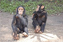
Two juvenile central chimpanzees, the nominate subspecies

In 2013 high resolution sequences were published from each of the four recognized chimpanzee subspecies: Central chimpanzee, Pan troglodytes troglodytes, 10 sequences; Western chimpanzee, Pan troglodytes verus, 6 sequences; Nigeria-Cameroon chimpanzee, Pan troglodytes ellioti, 4 sequences; and Eastern chimpanzee, Pan troglodytes schweinfurthii, 4 sequences. They were all sequenced to a mean of 25-fold coverage per individual.

The research showed considerable genome diversity in chimpanzees with many population-specific traits. The central chimpanzees retain the highest diversity in the chimpanzee lineage, whereas the other subspecies demonstrate signs of population bottlenecks.

Background

Human and chimpanzee chromosomes are very alike. The primary difference is that humans have one fewer pair of chromosomes than do other great apes. Humans have 23 pairs of chromosomes and other great apes have 24 pairs of chromosomes. In the human evolutionary lineage, two ancestral ape chromosomes fused at their telomeres, producing human chromosome 2. There are nine other major chromosomal differences between chimpanzees and humans: chromosome segment inversions on human chromosomes 1, 4, 5, 9, 12, 15, 16, 17, and 18. After the completion of the Human genome project, a common chimpanzee genome project was initiated. In December 2003, a preliminary analysis of 7600 genes shared between the two genomes confirmed that certain genes such as the forkhead-box P2 transcription factor, which is involved in speech development, are different in the human lineage. Several genes involved in hearing were also found to have changed during human evolution, suggesting selection involving human language-related behavior. Differences between individual humans and common chimpanzees are estimated to be about 10 times the typical difference between pairs of humans.

Another study showed that patterns of DNA methylation, which are a known regulation mechanism for gene expression, differ in the prefrontal cortex of humans versus chimpanzees, and implicated this difference in the evolutionary divergence of the two species.

Chimpanzee-human chromosome differences. A major structural difference is that human chromosome 2 (green color code) was derived from two smaller chromosomes that are found in other great apes (now called 2A and 2B ). Parts of human chromosome 2 are scattered among parts of several cat and rat chromosomes in these species that are more distantly related to humans (more ancient common ancestors; about 85 million years since the human/rodent common ancestor 

Draft genome sequence of the common chimpanzee

An analysis of the chimpanzee genome sequence was published in Nature on September 1, 2005, in an article produced by the Chimpanzee Sequencing and Analysis Consortium, a group of scientists which is supported in part by the National Human Genome Research Institute, one of the National Institutes of Health. The article marked the completion of the draft genome sequence.

A database now exists containing the genetic differences between human and chimpanzee genes, with about thirty-five million single-nucleotide changes, five million insertion/deletion events, and various chromosomal rearrangements. Gene duplications account for most of the sequence differences between humans and chimps. Single-base-pair substitutions account for about half as much genetic change as does gene duplication.

Typical human and chimpanzee homologs of proteins differ in only an average of two amino acids. About 30 percent of all human proteins are identical in sequence to the corresponding chimpanzee protein. As mentioned above, gene duplications are a major source of differences between human and chimpanzee genetic material, with about 2.7 percent of the genome now representing differences having been produced by gene duplications or deletions during approximately 6 million years since humans and chimpanzees diverged from their common evolutionary ancestor. The comparable variation within human populations is 0.5 percent.

About 600 genes were identified that may have been undergoing strong positive selection in the human and chimpanzee lineages; many of these genes are involved in immune system defense against microbial disease (example: granulysin is protective against Mycobacterium tuberculosis) or are targeted receptors of pathogenic microorganisms (example: Glycophorin C and Plasmodium falciparum). By comparing human and chimpanzee genes to the genes of other mammals, it has been found that genes coding for transcription factors, such as forkhead-box P2 (FOXP2), have often evolved faster in the human relative to chimpanzee; relatively small changes in these genes may account for the morphological differences between humans and chimpanzees. A set of 348 transcription factor genes code for proteins with an average of about 50 percent more amino acid changes in the human lineage than in the chimpanzee lineage.

Six human chromosomal regions were found that may have been under particularly strong and coordinated selection during the past 250,000 years. These regions contain at least one marker allele that seems unique to the human lineage while the entire chromosomal region shows lower than normal genetic variation. This pattern suggests that one or a few strongly selected genes in the chromosome region may have been preventing the random accumulation of neutral changes in other nearby genes. One such region on chromosome 7 contains the FOXP2 gene (mentioned above) and this region also includes the Cystic fibrosis transmembrane conductance regulator (CFTR) gene, which is important for ion transport in tissues such as the salt-secreting epithelium of sweat glands. Human mutations in the CFTR gene might be selected for as a way to survive cholera.

Another such region on chromosome 4 may contain elements regulating the expression of a nearby protocadherin gene that may be important for brain development and function. Although changes in expression of genes that are expressed in the brain tend to be less than for other organs (such as liver) on average, gene expression changes in the brain have been more dramatic in the human lineage than in the chimpanzee lineage. This is consistent with the dramatic divergence of the unique pattern of human brain development seen in the human lineage compared to the ancestral great ape pattern. The protocadherin-beta gene cluster on chromosome 5 also shows evidence of possible positive selection.

Results from the human and chimpanzee genome analyses should help in understanding some human diseases. Humans appear to have lost a functional Caspase 12 gene, which in other primates codes for an enzyme that may protect against Alzheimer's disease.

Human and chimpanzee genomes. M stands for Mitochondrial DNA

Genes of the chromosome 2 fusion site

Diagramatic representation of the location of the fusion site of chromosomes 2A and 2B and the genes inserted at this location.

The results of the chimpanzee genome project suggest that when ancestral chromosomes 2A and 2B fused to produce human chromosome 2, no genes were lost from the fused ends of 2A and 2B. At the site of fusion, there are approximately 150,000 base pairs of sequence not found in chimpanzee chromosomes 2A and 2B. Additional linked copies of the PGML/FOXD/CBWD genes exist elsewhere in the human genome, particularly near the p end of chromosome 9. This suggests that a copy of these genes may have been added to the end of the ancestral 2A or 2B prior to the fusion event. It remains to be determined if these inserted genes confer a selective advantage.

• PGM5P4. The phosphoglucomutase pseudogene of human chromosome 2. This gene is incomplete and doesn't produce a functional transcript.
• FOXD4L1. The forkhead box D4-like gene is an example of an intronless gene. The function of this gene is not known, but it may code for a transcription control protein.
• CBWD2. Cobalamin synthetase is a bacterial enzyme that makes vitamin B₁₂. In the distant past, a common ancestor to mice and apes incorporated a copy of a cobalamin synthetase gene (see: Horizontal gene transfer). Humans are unusual in that they have several copies of cobalamin synthetase-like genes, including the one on chromosome 2. It remains to be determined what the function of these human cobalamin synthetase-like genes is. If these genes are involved in vitamin B₁₂ metabolism, this could be relevant to human evolution. A major change in human development is greater post-natal brain growth than is observed in other apes. Vitamin B₁₂ is important for brain development, and vitamin B₁₂ deficiency during brain development results in severe neurological defects in human children.
• WASH2P. Several transcripts of unknown function corresponding to this region have been isolated. This region is also present in the closely related chromosome 9p terminal region that contains copies of the PGML/FOXD/CBWD genes.
• RPL23AP7. Many ribosomal protein L23a pseudogenes are scattered through the human genome.

Beef hormone controversy

From Wikipedia, the free encyclopedia
https://en.wikipedia.org/wiki/Beef_hormone_controversy

The beef hormone controversy or beef hormone dispute is one of the most intractable agricultural trade controversies since the establishment of the World Trade Organization (WTO).

It has sometimes been called the "beef war" in the media, as was the UK–EU beef dispute, creating some confusion, especially when both were occurring.

In 1989, the European Union banned the import of meat that contained artificial beef growth hormones approved for use and administered in the United States. Originally, the ban covered six such hormones but was amended in 2003 to permanently ban one hormone —estradiol-17β — while provisionally banning the use of the five others. WTO rules permit such bans, but only where a signatory presents valid scientific evidence that the ban is a health and safety measure. Canada and the United States opposed this ban, taking the EU to the WTO Dispute Settlement Body. In 1997, the WTO Dispute Settlement Body ruled against the EU.

History

EU ban and its background

The hormones banned by the EU in cattle farming were estradiol, progesterone, testosterone, zeranol, melengestrol acetate and trenbolone acetate. Of these, the first three are synthetic versions of endogenous hormones that are naturally produced in humans and animals, and also occur in a wide range of foods, whereas the last two are synthetic and not naturally occurring, which mimic the behaviour of endogenous hormones. Zeranol (alpha-zearalanol) is produced semi-synthetically, but it also occurs naturally in some foods. It is one of several derivatives of zearalenone produced by certain Fusarium. Although its occurrence in animal products can be partly due to its ingestion in such feeds, alpha-zearalanol can also be produced endogenously in ruminants that have ingested zearalenone and some zearalenone derivatives in such feeds. The EU did not impose an absolute ban. Under veterinary supervision, cattle farmers were permitted to administer the synthetic versions of natural hormones for cost-reduction and possibly therapeutic purposes, such as synchronising the oestrus cycles of dairy cows. All six hormones were licensed for use in the US and in Canada.

Under the Agreement on the Application of Sanitary and Phytosanitary Measures, signatories have the right to impose restrictions on health and safety grounds subject to scientific analysis. The heart of the Beef Hormone Dispute was the fact that all risk analysis is statistical in nature, and thus unable to determine with certainty the absence of health risks, and consequent disagreement between the US and Canada beef producers on the one hand, who believed that a broad scientific consensus existed that beef produced with the use of hormones was safe, and the EU on the other, which asserted that it was not safe.

The use of these hormones in cattle farming had been studied scientifically in North America for 50 years prior to the ban, and there had been widespread long-term use in over 20 countries. Canada and the United States asserted that this provided empirical evidence both of long-term safety and of scientific consensus.

The EU ban was not, as it was portrayed to rural constituencies in the US and Canada, protectionism. The EU had already had other measures that effectively restricted the import of North American beef. In the main, the North American product that the new ban affected, which existing barriers did not, was edible offal.

Consumers expressing concern over the safety of hormone use pressured EU officials. There were a series of widely publicized "hormone scandals" in Italy in the late 1970s and early 1980s. The first, in 1977, was signs of the premature onset of puberty in northern Italian schoolchildren, where investigators had cast suspicion in the direction of school lunches that had used meat farmed with the (illegal) use of growth hormones. No concrete evidence linking premature puberty to growth hormones was found, in part because no samples of the suspect meals were available for analysis. But public anger arose at the use of such meat production techniques, to be further fanned by the discovery in 1980 of the (again illegal) presence of diethylstilbestrol (DES), another synthetic hormone, in veal-based baby foods.

The scientific evidence for health risks associated with the use of growth hormones in meat production was, at best, scant. However, consumer lobbyist groups were far more able to successfully influence the European Parliament to enact regulations in the 1980s than producer lobbyist groups were, and had far more influence over public perceptions. This is in contrast with the US at the time, where there was little interest from consumer organizations in the subject prior to the 1980s, and regulations were driven by a well-organized coalition of export-oriented industry and farming interests, who were only opposed by traditional farming groups.

Until 1980, the use of growth hormones, both endogenous and exogenous, was completely prohibited in (as noted above) Italy, Denmark, the Netherlands, and Greece. Germany, the largest beef producer in the EU at the time, prohibited just the use of exogenous growth hormones. The five other member countries, including the second and third largest beef producers, France and the United Kingdom, permitted their use. (The use of growth hormones was particularly common in the U.K., where beef production was heavily industrialized.) This had resulted in several disputes amongst member countries, with the countries that had no prohibitions arguing that the restrictions by the others acted as non-tariff trade barriers. But in response to the public outcry in 1980, in combination with the contemporary discovery that DES was a teratogen, the EU began to issue regulations, beginning with a directive prohibiting the use of stilbenes and thyrostatics issued by the European Community Council of Agriculture Ministers in 1980, and the commissioning of a scientific study into the use of estradiol, testosterone, progesterone, trenbolone, and zeranol in 1981.

The European Consumers' Organisation (BEUC) lobbied for a total ban upon growth hormones, opposed, with only partial success, by the pharmaceutical industry, which was not well organized at the time. (It was not until 1987, at the instigation of US firms, that the European Federation of Animal Health, FEDESA, was formed to represent at EU level the companies that, amongst other things, manufactured growth hormones.) Neither European farmers nor the meat processing industry took any stance on the matter. With the help of the BEUC consumer boycotts of veal products, sparked in Italy by reports about DES in Italian magazines and in France and Germany by similar reports, spread from those three countries across the whole of the EU, causing companies such as Hipp and Alete to withdraw their lines of veal products, and veal prices to drop significantly in France, Belgium, West Germany, Ireland, and the Netherlands. Because of the fixed purchases guaranteed by the EU's Common Agricultural Policy, there was a loss of ECU 10 million to the EU's budget.

The imposition of a general ban was encouraged by the European Parliament, with a 1981 resolution passing by a majority of 177:1 in favour of a general ban. MEPs, having been directly elected for the first time in 1979, were taking the opportunity to flex their political muscles, and were in part using the public attention on the issue to strengthen the Parliament's role. The Council of Ministers was divided along lines that directly matched each country's domestic stance on growth hormone regulation, with France, Ireland, the U.K., Belgium, Luxembourg, and Germany all opposing a general ban. The European Commission, leery of a veto by the Council and tightly linked to both pharmaceutical and (via Directorate VI) agricultural interests, presented factual arguments and emphasized the problem of trade barriers.

1998 WTO decision

The WTO Appellate Body affirmed the WTO Panel conclusion in a report adopted by the WTO Dispute Settlement Body on 13 February 1998. Section 208 of this report says:

[W]e find that the European Communities did not actually proceed to an assessment, within the meaning of Articles 5.1 and 5.2, of the risks arising from the failure of observance of good veterinary practice combined with problems of control of the use of hormones for growth promotion purposes. The absence of such risk assessment, when considered in conjunction with the conclusion actually reached by most, if not all, of the scientific studies relating to the other aspects of risk noted earlier, leads us to the conclusion that no risk assessment that reasonably supports or warrants the import prohibition embodied in the EC Directives was furnished to the Panel. We affirm, therefore, the ultimate conclusions of the Panel that the EC import prohibition is not based on a risk assessment within the meaning of Articles 5.1 and 5.2 of the SPS Agreement and is, therefore, inconsistent with the requirements of Article 5.1.

On 12 July 1999, an arbitrator appointed by the WTO Dispute Settlement Body authorized the US to impose retaliatory tariffs of US$116.8 million per year on the EU.

EU scientific risk assessments

In 2002 the EU Scientific Committee on Veterinary Measures relating to Public Health (SCVPH) claimed that the use of beef growth hormones posed a potential health risk, and in 2003 the EU enacted Directive 2003/74/EC to amend its ban, but the US and Canada rejected that the EU had met WTO standards for scientific risk assessment.

The EC made the scientific claim that the hormones used in treating cattle remain in the tissue, specifically the hormone 17-beta estradiol. However, despite this evidence the EC declared there was no clear link to health risks in humans for the other five provisionally banned hormones. The EC has also found high amounts of hormones in areas where there are dense cattle lots. This increase in hormones in the water has affected waterways and nearby wild fish. Contamination of North American waterways by hormones would not, however, have any direct impact on European consumers or their health.

2008 WTO decision

In November 2004, the EU requested WTO consultations, claiming that the United States should remove its retaliatory measures since the EU has removed the measures found to be WTO-inconsistent in the original case. In 2005, the EU initiated new WTO dispute settlement proceedings against the United States and Canada, and a March 2008 panel report cited fault with all three parties (EU, United States, and Canada) on various substantive and procedural aspects of the dispute. In October 2008, the WTO Appellate Body issued a mixed ruling that allows for continued imposition of trade sanctions on the EU by the United States and Canada, but also allows the EU to continue its ban on imports of hormone-treated beef.

In November 2008, the EU filed a new WTO challenge following the announcement by the USTR that it was seeking comment on possible modification of the list of EU products subject to increased tariffs under the dispute, and in January 2009 the USTR announced changes to the list of EU products subject to increased tariffs. In September 2009, the United States and the European Commission signed a memorandum of understanding, which established a new EU duty-free import quota for grain-fed, high quality beef (HQB) as part of a compromise solution. However, in December 2016, the US took steps to reinstate retaliatory tariffs on the list of EU products under the dispute given continued concerns about US beef access to the EU market, and in August 2019 they agreed establishing an initial duty-free tariff-rate quota of 18,500 tonnes annually, phased over seven years to 35,000 tonnes (valued at approximately US$420 million) of the EU 45,000 tonnes quota of non-hormone treated beef.

Effects upon policy in the EU

The EU often applies the precautionary principle very stringently in regards to food safety. The precautionary principle means that in a case of scientific uncertainty, the government may take appropriate measures proportionate to the potential risk (EC Regulation 178/2002). In 1996, the EU banned imported beef from the US and continued to do so after the 2003 Mad Cow scare. A more sophisticated risk assessment found there to be insufficient risk to ban certain hormones, but continued to ban others. Labeling of meat was another option, however warnings were also insufficient because of the criteria specified in the SPS (Sanitary and Phyto-Sanitary agreement). This agreement allows members to use scientifically based measures to protect public health. Most specifically the Equivalence provision in Article 4 which states the following: "an importing country must accept an SPS measure which differs from its own as equivalent if the exporting country’s measure provides the same level of health or environmental protection." Therefore, although the EU is a strong proponent of labels and banning meat that contains growth hormones, requiring the US to do the same would have violated this agreement.

Effects upon public opinion in the US

One of the effects of the Beef Hormone Dispute in the US was to awaken the public's interest in the issue. This interest was not wholly unsympathetic to the EU. In 1989, for example, the Consumer Federation of America and the Center for Science in the Public Interest both pressed for an adoption of a ban within the US similar to that within the EU. US consumers appear to be less concerned with the use of synthetic chemicals in food production. Because of current policy, in which all beef is allowed whether produced with hormones or genetically modified, US consumers now have to rely on their own judgment when buying goods. However, in a study done in 2002, 85% of respondents wanted mandatory labeling on beef produced with growth hormones. The public in general is motivated to purchase organic or natural meats for several reasons. Organic meats and poultry is the fastest growing agricultural sector; from 2002 to 2003 there was a growth of 77.8%, accounting for $23 billion in the entire organic food market.

Feed conversion ratio

From Wikipedia, the free encyclopedia

https://en.wikipedia.org/wiki/Feed_conversion_ratio

In animal husbandry, feed conversion ratio (FCR) or feed conversion rate is a ratio or rate measuring of the efficiency with which the bodies of livestock convert animal feed into the desired output. For dairy cows, for example, the output is milk, whereas in animals raised for meat (such as beef cows, pigs, chickens, and fish) the output is the flesh, that is, the body mass gained by the animal, represented either in the final mass of the animal or the mass of the dressed output. FCR is the mass of the input divided by the output (thus mass of feed per mass of milk or meat). In some sectors, feed efficiency, which is the output divided by the input (i.e. the inverse of FCR), is used. These concepts are also closely related to efficiency of conversion of ingested foods (ECI).

Background

Feed conversion ratio (FCR) is the ratio of inputs to outputs; it is the inverse of "feed efficiency" which is the ratio of outputs to inputs. FCR is widely used in hog and poultry production, while FE is used more commonly with cattle. Being a ratio the FCR is dimensionless, that is, it is not affected by the units of measurement used to determine the FCR.

FCR a function of the animal's genetics and age, the quality and ingredients of the feed, and the conditions in which the animal is kept, and storage and use of the feed by the farmworkers.

As a rule of thumb, the daily FCR is low for young animals (when relative growth is large) and increases for older animals (when relative growth tends to level out). However FCR is a poor basis to use for selecting animals to improve genetics, as that results in larger animals that cost more to feed; instead residual feed intake (RFI) is used which is independent of size. RFI uses for output the difference between actual intake and predicted intake based on an animal's body weight, weight gain, and composition.

The outputs portion may be calculated based on weight gained, on the whole animal at sale, or on the dressed product; with milk it may be normalized for fat and protein content.

As for the inputs portion, although FCR is commonly calculated using feed dry mass, it is sometimes calculated on an as-fed wet mass basis, (or in the case of grains and oilseeds, sometimes on a wet mass basis at standard moisture content), with feed moisture resulting in higher ratios.

Conversion ratios for livestock

Animals that have a low FCR are considered efficient users of feed. However, comparisons of FCR among different species may be of little significance unless the feeds involved are of similar quality and suitability.

Beef cattle

As of 2013 in the US, an FCR calculated on live weight gain of 4.5–7.5 was in the normal range with an FCR above 6 being typical. Divided by an average carcass yield of 62.2%, the typical carcass weight FCR is above 10. As of 2013 FCRs had not changed much compared to other fields in the prior 30 years, especially compared to poultry which had improved feed efficiency by about 250% over the last 50 years.

Dairy cattle

The dairy industry traditionally didn't use FCR but in response to increasing concentration in the dairy industry and other livestock operations, the EPA updated its regulations in 2003 controlling manure and other waste releases produced by livestock operators. In response the USDA began issuing guidance to dairy farmers about how to control inputs to better minimize manure output and to minimize harmful contents, as well as optimizing milk output.

In the US, the price of milk is based on the protein and fat content, so the FCR is often calculated to take that into account. Using an FCR calculated just on the weight of protein and fat, as of 2011 an FCR of 13 was poor, and an FCR of 8 was very good.

Another method for dealing with pricing based on protein and fat, is using energy-corrected milk (ECM), which adds a factor to normalize assuming certain amounts of fat and protein in a final milk product; that formula is (0.327 x milk mass) + (12.95 x fat mass) + (7.2 x protein mass).

In the dairy industry, feed efficiency (ECM/intake) is often used instead of FCR (intake/ECM); an FE less than 1.3 is considered problematic.

FE based simply on the weight of milk is also used; an FE between 1.30 and 1.70 is normal.

Pigs

Pigs have been kept to produce meat for 5,000 to 9,000 years. As of 2011, pigs used commercially in the UK and Europe had an FCR, calculated using weight gain, of about 1 as piglets and ending about 3 at time of slaughter. As of 2012 in Australia and using dressed weight for the output, a FCR calculated using weight of dressed meat of 4.5 was fair, 4.0 was considered "good", and 3.8, "very good".

The FCR of pigs is greatest up to the period, when pigs weigh 220 pounds. During this period, their FCR is 3.5. Their FCR begins decreasing gradually after this period. For instance, in the US as of 2012, commercial pigs had FCR calculated using weight gain, of 3.46 for while they weighed between 240 and 250 pounds, 3.65 between 250 and 260 pounds, 3.87 between 260 and 270 lbs, and 4.09 between 280 and 270 lbs.

Because FCR calculated on the basis of weight gained gets worse after pigs mature, as it takes more and more feed to drive growth, countries that have a culture of slaughtering pigs at very high weights, like Japan and Korea, have poor FCRs.

Sheep

Some data for sheep illustrate variations in FCR. A FCR (kg feed dry matter intake per kg live mass gain) for lambs is often in the range of about 4 to 5 on high-concentrate rations, 5 to 6 on some forages of good quality, and more than 6 on feeds of lesser quality. On a diet of straw, which has a low metabolizable energy concentration, FCR of lambs may be as high as 40. Other things being equal, FCR tends to be higher for older lambs (e.g. 8 months) than younger lambs (e.g. 4 months).

Poultry

As of 2011 in the US, broiler chickens has an FCR of 1.6 based on body weight gain, and mature in 39 days. At around the same time the FCR based on weight gain for broilers in Brazil was 1.8. The global average in 2013 is around 2.0 for weight gain (live weight) and 2.8 for slaughtered meat (carcass weight).

For hens used in egg production in the US, as of 2011 the FCR was about 2, with each hen laying about 330 eggs per year. When slaughtered, the world average layer flock as of 2013 yields a carcass FCR of 4.2, still much better than the average backyard chicken flock (FCR 9.2 for eggs, 14.6 for carcass).

From the early 1960s to 2011 in the US broiler growth rates doubled and their FCRs halved, mostly due to improvements in genetics and rapid dissemination of the improved chickens. The improvement in genetics for growing meat created challenges for farmers who breed the chickens that are raised by the broiler industry, as the genetics that cause fast growth decreased reproductive abilities.

Carnivorous fish

The FIFO ratio (or Fish In – Fish Out ratio) is a conversion ratio applied to aquaculture, where the first number is the mass of harvested fish used to feed farmed fish, and the second number is the mass of the resulting farmed fish. FIFO is a way of expressing the contribution from harvested wild fish used in aquafeed compared with the amount of edible farmed fish, as a ratio. Fishmeal and fish oil inclusion rates in aquafeeds have shown a continual decline over time as aquaculture grows and more feed is produced, but with a finite annual supply of fishmeal and fish oil. Calculations have shown that the overall fed aquaculture FIFO declined from 0.63 in 2000 to 0.33 in 2010, and 0.22 in 2015. In 2015, therefore, approximately 4.55 kg of farmed fish was produced for every 1 kg of wild fish harvested and used in feed. The fish used in fishmeal and fish oil production are not used for human consumption, but with their use as fishmeal and fish oil in aquafeed they contribute to global food production.

As of 2015 farm raised Atlantic salmon had a commodified feed supply with four main suppliers, and an FCR of around 1. Tilapia is about 1.5, and as of 2013 farmed catfish had a FCR of about 1.

Herbivorous and omnivorous fish

For herbivorous and omnivorous fish like Chinese carp and tilapia, the plant-based feed yields much lower FCR compared to carnivorous kept on a partially fish-based diet, despite a decrease in overall resource use. The edible (fillet) FCR of tilapia is around 4.6 and the FCR of Chinese carp is around 4.9.

Rabbits

In India, rabbits raised for meat had an FCR of 2.5 to 3.0 on high grain diet and 3.5 to 4.0 on natural forage diet, without animal-feed grain.

Global averages by species and production systems

In a global study published in the journal Global Food Security, FAO estimated various feed conversion ratios, taking into account the diversity of feed material consumed by livestock. At global level, ruminants require 133 kg of dry matter per kg of protein while monograstrics require 30. However, when considering human edible feed only, ruminants require 5.9 kg of feed to produce 1 kg of animal protein, while monogatrsics require 15.8 kg. When looking at meat only, ruminants consume an average of 2.8 kg of human edible feed per kg of meat produced, while monogastrics need 3.2. Finally, when accounting for the protein content of the feed, ruminant need an average of 0.6 kg of edible plant protein to produce 1 kg of animal protein while monogastric need 2. This means that ruminants make a positive net contribution to the supply of edible protein for humans at global level.

Feed conversion ratios of meat alternatives

Many alternatives to conventional animal meat sources have been proposed for higher efficiency, including insects, meat analogues, and cultured meats.

Insects

Although there are few studies of the feed conversion ratios of edible insects, the house cricket (Acheta domesticus) has been shown to have a FCR of 0.9 - 1.1 depending on diet composition. A more recent work gives an FCR of 1.9–2.4. Reasons contributing to such a low FCR include the whole body being used for food, the lack of internal temperature control (insects are poikilothermic), high fecundity and rate of maturation.

Meat analogue

If one treats tofu as a meat, the FCR reaches as low as 0.29. The FCRs for less watery forms of meat analogues are unknown.

Cultured meat

Although cultured meat has a potentially much lower land footprint required, its FCR is closer to poultry at around 4 (2-8). It has a high need for energy inputs.