North Atlantic oscillation

From Wikipedia, the free encyclopedia

https://en.wikipedia.org/wiki/Atlantic_multidecadal_oscillation

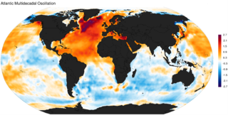
Atlantic multidecadal oscillation spatial pattern obtained as the regression of monthly HadISST sea surface temperature anomalies (1870–2013).

Atlantic Multidecadal Oscillation Index according to the methodology proposed by van Oldenborgh et al. 1880–2018.

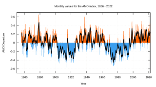
Atlantic Multidecadal Oscillation index computed as the linearly detrended North Atlantic sea surface temperature anomalies 1856–2022.

The Atlantic Multidecadal Oscillation (AMO), also known as Atlantic Multidecadal Variability (AMV), is the theorized variability of the sea surface temperature (SST) of the North Atlantic Ocean on the timescale of several decades.

While there is some support for this mode in models and in historical observations, controversy exists with regard to its amplitude, and whether it has a typical timescale and can be classified as an oscillation. There is also discussion on the attribution of sea surface temperature change to natural or anthropogenic causes, especially in tropical Atlantic areas important for hurricane development. The Atlantic multidecadal oscillation is also connected with shifts in hurricane activity, rainfall patterns and intensity, and changes in fish populations.

Definition and history

Evidence for a multidecadal climate oscillation centered in the North Atlantic began to emerge in 1980s work by Folland and colleagues, seen in Fig. 2.d.A. That oscillation was the sole focus of Schlesinger and Ramankutty in 1994, but the actual term Atlantic Multidecadal Oscillation (AMO) was coined by Michael Mann in a 2000 telephone interview with Richard Kerr, as recounted by Mann, p. 30 in The Hockey Stick and the Climate Wars: Dispatches from the Front Lines (2012).

The AMO signal is usually defined from the patterns of SST variability in the North Atlantic once any linear trend has been removed. This detrending is intended to remove the influence of greenhouse gas-induced global warming from the analysis. However, if the global warming signal is significantly non-linear in time (i.e. not just a smooth linear increase), variations in the forced signal will leak into the AMO definition. Consequently, correlations with the AMO index may mask effects of global warming, as per Mann, Steinman and Miller, which also provides a more detailed history of the science development.

AMO index

Several methods have been proposed to remove the global trend and El Niño-Southern Oscillation (ENSO) influence over the North Atlantic SST. Trenberth and Shea, assuming that the effect of global forcing over the North Atlantic is similar to the global ocean, subtracted the global (60°N-60°S) mean SST from the North Atlantic SST to derive a revised AMO index.

Ting et al. however argue that the forced SST pattern is not globally uniform; they separated the forced and internally generated variability using signal to noise maximizing EOF analysis.

Van Oldenborgh et al. derived an AMO index as the SST averaged over the extra-tropical North Atlantic (to remove the influence of ENSO that is greater at tropical latitude) minus the regression on global mean temperature.

Guan and Nigam removed the non stationary global trend and Pacific natural variability before applying an EOF analysis to the residual North Atlantic SST.

The linearly detrended index suggests that the North Atlantic SST anomaly at the end of the twentieth century is equally divided between the externally forced component and internally generated variability, and that the current peak is similar to middle twentieth century; by contrast the others methodology suggest that a large portion of the North Atlantic anomaly at the end of the twentieth century is externally forced.

Frajka-Williams et al. 2017 pointed out that recent changes in cooling of the subpolar gyre, warm temperatures in the subtropics and cool anomalies over the tropics, increased the spatial distribution of meridional gradient in sea surface temperatures, which is not captured by the AMO Index.

Mechanisms

See also: Atlantic meridional overturning circulation and Ocean heat content

Based on the about 150-year instrumental record a quasi-periodicity of about 70 years, with a few distinct warmer phases between ca. 1930–1965 and after 1995, and cool between 1900–1930 and 1965–1995 has been identified. In models, AMO-like variability is associated with small changes in the North Atlantic branch of the Thermohaline Circulation. However, historical oceanic observations are not sufficient to associate the derived AMO index to present-day circulation anomalies. Models and observations indicate that changes in atmospheric circulation, which induce changes in clouds, atmospheric dust and surface heat flux, are largely responsible for the tropical portion of the AMO.

The Atlantic Multidecadal Oscillation (AMO) is important for how external forcings are linked with North Atlantic SSTs.

Climate impacts worldwide

The AMO is correlated to air temperatures and rainfall over much of the Northern Hemisphere, in particular in the summer climate in North America and Europe. Through changes in atmospheric circulation, the AMO can also modulate spring snowfall over the Alps and glaciers' mass variability. Rainfall patterns are affected in North Eastern Brazilian and African Sahel. It is also associated with changes in the frequency of North American droughts and is reflected in the frequency of severe Atlantic hurricane activity.

Recent research suggests that the AMO is related to the past occurrence of major droughts in the US Midwest and the Southwest. When the AMO is in its warm phase, these droughts tend to be more frequent or prolonged. Two of the most severe droughts of the 20th century occurred during the positive AMO between 1925 and 1965: The Dust Bowl of the 1930s and the 1950s drought. Florida and the Pacific Northwest tend to be the opposite—warm AMO, more rainfall.

Climate models suggest that a warm phase of the AMO strengthens the summer rainfall over India and Sahel and the North Atlantic tropical cyclone activity. Paleoclimatologic studies have confirmed this pattern—increased rainfall in AMO warmphase, decreased in cold phase—for the Sahel over the past 3,000 years.

Relation to Atlantic hurricanes

See also: Tropical cyclones and climate change

North Atlantic tropical cyclone activity according to the Accumulated Cyclone Energy Index, 1950–2015.

A 2008 study correlated the Atlantic Multidecadal Mode (AMM), with HURDAT data (1851–2007), and noted a positive linear trend for minor hurricanes (category 1 and 2), but removed when the authors adjusted their model for undercounted storms, and stated "If there is an increase in hurricane activity connected to a greenhouse gas induced global warming, it is currently obscured by the 60 year quasi-periodic cycle." With full consideration of meteorological science, the number of tropical storms that can mature into severe hurricanes is much greater during warm phases of the AMO than during cool phases, at least twice as many; the AMO is reflected in the frequency of severe Atlantic hurricanes. Based on the typical duration of negative and positive phases of the AMO, the current warm regime is expected to persist at least until 2015 and possibly as late as 2035. Enfield et al. assume a peak around 2020.

However, Mann and Emanuel had found in 2006 that "anthropogenic factors are responsible for long-term trends in tropic Atlantic warmth and tropical cyclone activity" and "There is no apparent role of the AMO."

In 2014 Mann, Steinman and Miller showed that warming (and therefore any effects on hurricanes) were not caused by the AMO, writing: "certain procedures used in past studies to estimate internal variability, and in particular, an internal multidecadal oscillation termed the "Atlantic Multidecadal Oscillation" or "AMO", fail to isolate the true internal variability when it is a priori known. Such procedures yield an AMO signal with an inflated amplitude and biased phase, attributing some of the recent NH mean temperature rise to the AMO. The true AMO signal, instead, appears likely to have been in a cooling phase in recent decades, offsetting some of the anthropogenic warming."

Periodicity and prediction of AMO shifts

There are only about 130–150 years of data based on instrument data, which are too few samples for conventional statistical approaches. With the aid of multi-century proxy reconstruction, a longer period of 424 years was used by Enfield and Cid–Serrano as an illustration of an approach as described in their paper called "The Probabilistic Projection of Climate Risk". Their histogram of zero crossing intervals from a set of five re-sampled and smoothed version of Gray et al. (2004) index together with the maximum likelihood estimate gamma distribution fit to the histogram, showed that the largest frequency of regime interval was around 10–20 year. The cumulative probability for all intervals 20 years or less was about 70%.

There is no demonstrated predictability for when the AMO will switch, in any deterministic sense. Computer models, such as those that predict El Niño, are far from being able to do this. Enfield and colleagues have calculated the probability that a change in the AMO will occur within a given future time frame, assuming that historical variability persists. Probabilistic projections of this kind may prove to be useful for long-term planning in climate sensitive applications, such as water management.

A 2017 study predicts a continued cooling shift beginning 2014, and the authors note, "..unlike the last cold period in the Atlantic, the spatial pattern of sea surface temperature anomalies in the Atlantic is not uniformly cool, but instead has anomalously cold temperatures in the subpolar gyre, warm temperatures in the subtropics and cool anomalies over the tropics. The tripole pattern of anomalies has increased the subpolar to subtropical meridional gradient in SSTs, which are not represented by the AMO index value, but which may lead to increased atmospheric baroclinicity and storminess."

Criticism

In a 2021 study by Michael Mann and others, it was shown that the periodicity of the AMO in the last millennium was driven by volcanic eruptions and other external forcings, and therefore that there is no compelling evidence for the AMO being an oscillation or cycle. There was also a lack of oscillatory behaviour in models on time scales longer than El Niño Southern Oscillation; the AMV is indistinguishable from red noise, a typical null hypothesis to test whether there are oscillations in a model. Referring to the 2021 study, Michael Mann, the originator of the term AMO, put it more succinctly in a blog post on the matter: "my colleagues and I have provided what we consider to be the most definitive evidence yet that the AMO doesn't actually exist."

Pacific decadal oscillation

From Wikipedia, the free encyclopedia
https://en.wikipedia.org/wiki/Pacific_decadal_oscillation

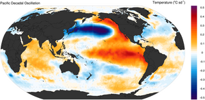
PDO positive phase global pattern

The Pacific decadal oscillation (PDO) is a robust, recurring pattern of ocean-atmosphere climate variability centered over the mid-latitude Pacific basin. The PDO is detected as warm or cool surface waters in the Pacific Ocean, north of 20°N. Over the past century, the amplitude of this climate pattern has varied irregularly at interannual-to-interdecadal time scales (meaning time periods of a few years to as much as time periods of multiple decades). There is evidence of reversals in the prevailing polarity (meaning changes in cool surface waters versus warm surface waters within the region) of the oscillation occurring around 1925, 1947, and 1977; the last two reversals corresponded with dramatic shifts in salmon production regimes in the North Pacific Ocean. This climate pattern also affects coastal sea and continental surface air temperatures from Alaska to California.

During a "warm", or "positive", phase, the west Pacific becomes cooler and part of the eastern ocean warms; during a "cool", or "negative", phase, the opposite pattern occurs. The Pacific decadal oscillation was named by Steven R. Hare, who noticed it while studying salmon production pattern results in 1997.

The Pacific decadal oscillation index is the leading empirical orthogonal function (EOF) of monthly sea surface temperature anomalies (SST-A) over the North Pacific (poleward of 20°N) after the global average sea surface temperature has been removed. This PDO index is the standardized principal component time series. A PDO 'signal' has been reconstructed as far back as 1661 through tree-ring chronologies in the Baja California area.

Mechanisms

Several studies have indicated that the PDO index can be reconstructed as the superimposition of tropical forcing and extra-tropical processes. Thus, unlike El Niño–Southern Oscillation (ENSO), the PDO is not a single physical mode of ocean variability, but rather the sum of several processes with different dynamic origins.

At inter-annual time scales the PDO index is reconstructed as the sum of random and ENSO induced variability in the Aleutian Low, whereas on decadal timescales ENSO teleconnections, stochastic atmospheric forcing and changes in the North Pacific oceanic gyre circulation contribute approximately equally. Additionally sea surface temperature anomalies have some winter to winter persistence due to the reemergence mechanism.

ENSO teleconnections, the atmospheric bridge

The atmospheric bridge during El Niño

ENSO can influence the global circulation pattern thousands of kilometers away from the equatorial Pacific through the "atmospheric bridge". During El Niño events, deep convection and heat transfer to the troposphere is enhanced over the anomalously warm sea surface temperature, this ENSO-related tropical forcing generates Rossby waves that propagate poleward and eastward and are subsequently refracted back from the pole to the tropics. The planetary waves form at preferred locations both in the North and South Pacific Ocean, and the teleconnection pattern is established within 2–6 weeks. ENSO driven patterns modify surface temperature, humidity, wind, and the distribution of clouds over the North Pacific that alter surface heat, momentum, and freshwater fluxes and thus induce sea surface temperature, salinity, and mixed layer depth (MLD) anomalies.

The atmospheric bridge is more effective during boreal winter when the deepened Aleutian Low results in stronger and cold northwesterly winds over the central Pacific and warm/humid southerly winds along the North American west coast, the associated changes in the surface heat fluxes and to a lesser extent Ekman transport creates negative sea surface temperature anomalies and a deepened MLD in the central Pacific and warm the ocean from the Hawaii to the Bering Sea.

SST reemergence

Reemergence mechanism in the North Pacific.

 

Mixed layer depth seasonal cycle.

Midlatitude SST anomaly patterns tend to recur from one winter to the next but not during the intervening summer, this process occurs because of the strong mixed layer seasonal cycle. The mixed layer depth over the North Pacific is deeper, typically 100-200m, in winter than it is in summer and thus SST anomalies that form during winter and extend to the base of the mixed layer are sequestered beneath the shallow summer mixed layer when it reforms in late spring and are effectively insulated from the air-sea heat flux. When the mixed layer deepens again in the following autumn/early winter the anomalies may again influence the surface. This process has been named "reemergence mechanism" by Alexander and Deser and is observed over much of the North Pacific Ocean although it is more effective in the west where the winter mixed layer is deeper and the seasonal cycle greater.

Stochastic atmospheric forcing

Long term sea surface temperature variation may be induced by random atmospheric forcings that are integrated and reddened into the ocean mixed layer. The stochastic climate model paradigm was proposed by Frankignoul and Hasselmann, in this model a stochastic forcing represented by the passage of storms alter the ocean mixed layer temperature via surface energy fluxes and Ekman currents and the system is damped due to the enhanced (reduced) heat loss to the atmosphere over the anomalously warm (cold) SST via turbulent energy and longwave radiative fluxes, in the simple case of a linear negative feedback the model can be written as the separable ordinary differential equation: ${\displaystyle \frac{\mathrm{d}y}{\mathrm{d}t}=v(t)-\lambda y}$

where v is the random atmospheric forcing, λ is the damping rate (positive and constant) and y is the response.

The variance spectrum of y is: ${\displaystyle G(w)=\frac{F}{w^2+{\lambda }^2}}$

where F is the variance of the white noise forcing and w is the frequency, an implication of this equation is that at short time scales (w>>λ) the variance of the ocean temperature increase with the square of the period while at longer timescales(w<<λ, ~150 months) the damping process dominates and limits sea surface temperature anomalies so that the spectra became white.

Thus an atmospheric white noise generates SST anomalies at much longer timescales but without spectral peaks. Modeling studies suggest that this process contribute to as much as 1/3 of the PDO variability at decadal timescales.

Ocean dynamics

Several dynamic oceanic mechanisms and SST-air feedback may contribute to the observed decadal variability in the North Pacific Ocean. SST variability is stronger in the Kuroshio Oyashio extension (KOE) region and is associated with changes in the KOE axis and strength, that generates decadal and longer time scales SST variance but without the observed magnitude of the spectral peak at ~10 years, and SST-air feedback. Remote reemergence occurs in regions of strong current such as the Kuroshio extension and the anomalies created near the Japan may reemerge the next winter in the central pacific.

Advective resonance

Saravanan and McWilliams have demonstrated that the interaction between spatially coherent atmospheric forcing patterns and an advective ocean shows periodicities at preferred time scales when non-local advective effects dominate over the local sea surface temperature damping. This "advective resonance" mechanism may generate decadal SST variability in the Eastern North Pacific associated with the anomalous Ekman advection and surface heat flux.

North Pacific oceanic gyre circulation

Dynamic gyre adjustments are essential to generate decadal SST peaks in the North Pacific, the process occurs via westward propagating oceanic Rossby waves that are forced by wind anomalies in the central and eastern Pacific Ocean. The quasi-geostrophic equation for long non-dispersive Rossby Waves forced by large scale wind stress can be written as the linear partial differential equation: ${\displaystyle \frac{\mathrm{\partial }h}{\mathrm{\partial }t}-c\frac{\mathrm{\partial }h}{\mathrm{\partial }x}=\frac{-\mathrm{\nabla }\times \overrightarrow{\tau }}{{\rho }_0{f}_0}}$

where h is the upper-layer thickness anomaly, τ is the wind stress, c is the Rossby wave speed that depends on latitude, ρ₀ is the density of sea water and f₀ is the Coriolis parameter at a reference latitude. The response time scale is set by the Rossby waves speed, the location of the wind forcing and the basin width, at the latitude of the Kuroshio Extension c is 2.5 cm s⁻¹ and the dynamic gyre adjustment timescale is ~(5)10 years if the Rossby wave was initiated in the (central)eastern Pacific Ocean.

If the wind white forcing is zonally uniform it should generate a red spectrum in which h variance increases with the period and reaches a constant amplitude at lower frequencies without decadal and interdecadal peaks, however low frequencies atmospheric circulation tends to be dominated by fixed spatial patterns so that wind forcing is not zonally uniform, if the wind forcing is zonally sinusoidal then decadal peaks occurs due to resonance of the forced basin-scale Rossby waves.

The propagation of h anomalies in the western pacific changes the KOE axis and strength and impact SST due to the anomalous geostrophic heat transport. Recent studies suggest that Rossby waves excited by the Aleutian low propagate the PDO signal from the North Pacific to the KOE through changes in the KOE axis while Rossby waves associated with the NPO propagate the North Pacific Gyre oscillation signal through changes in the KOE strength.

Impacts

Temperature and precipitation

PDO DJFM temperature pattern.

 

PDO DJFM precipitation pattern.

The PDO spatial pattern and impacts are similar to those associated with ENSO events. During the positive phase the wintertime Aleutian Low is deepened and shifted southward, warm/humid air is advected along the North American west coast and temperatures are higher than usual from the Pacific Northwest to Alaska but below normal in Mexico and the Southeastern United States.
Winter precipitation is higher than usual in the Alaska Coast Range, Mexico and the Southwestern United States but reduced over Canada, Eastern Siberia and Australia.
McCabe et al. showed that the PDO along with the AMO strongly influence multidecadal droughts pattern in the United States, drought frequency is enhanced over much of the Northern United States during the positive PDO phase and over the Southwest United States during the negative PDO phase in both cases if the PDO is associated with a positive AMO.
The Asian Monsoon is also affected, increased rainfall and decreased summer temperature is observed over the Indian subcontinent during the negative phase.

PDO Indicators	PDO positive phase	PDO negative phase
Temperature
Pacific Northwest, British Columbia, and Alaska	Above average	Below average
Mexico to South-East US	Below average	Above average
Precipitation
Alaska coastal range	Above average	Below average
Mexico to South-Western US	Above average	Below average
Canada, Eastern Siberia and Australia	Below average	Above average
India summer monsoon	Below average	Above average

Reconstructions and regime shifts

Observed monthly values for the PDO (1900–sep2019, dots) and 10-year averages.

 

Reconstructed PDO Index (993-1996).

The PDO index has been reconstructed using tree rings and other hydrologically sensitive proxies from west North America and Asia.

MacDonald and Case reconstructed the PDO back to 993 using tree rings from California and Alberta. The index shows a 50–70 year periodicity but is a strong mode of variability only after 1800, a persistent negative phase occurring during medieval times (993–1300) which is consistent with La Niña conditions reconstructed in the tropical Pacific and multi-century droughts in the South-West United States.

Several regime shifts are apparent both in the reconstructions and instrumental data, during the 20th century regime shifts associated with concurrent changes in SST, SLP, land precipitation and ocean cloud cover occurred in 1924/1925, 1945/1946, and 1976/1977:

• 1750: PDO displays an unusually strong oscillation.
• 1924/1925: PDO changed to a "warm" phase.
• 1945/1946: The PDO changed to a "cool" phase, the pattern of this regime shift is similar to the 1970s episode with maximum amplitude in the subarctic and subtropical front but with a greater signature near the Japan while the 1970s shift was stronger near the American west coast.
• 1976/1977: PDO changed to a "warm" phase.
• 1988/1989: A weakening of the Aleutian low with associated SST changes was observed, in contrast to others regime shifts this change appears to be related to concurrent extratropical oscillation in the North Pacific and North Atlantic rather than tropical processes.
• 1997/1998: Several changes in sea surface temperature and marine ecosystem occurred in the North Pacific after 1997/1998, in contrast to prevailing anomalies observed after the 1970s shift. The SST declined along the United States west coast and substantial changes in the populations of salmon, anchovy and sardine were observed as the PDO changed back to a cool "anchovy" phase. However the spatial pattern of the SST change was different with a meridional SST seesaw in the central and western Pacific that resembled a strong shift in the North Pacific Gyre Oscillation rather than the PDO structure. This pattern dominated much of the North Pacific SST variability after 1989.
• The 2014 flip from the cool PDO phase to the warm phase, which vaguely resembles a long and drawn-out El Niño event, contributed to record-breaking surface temperatures across the planet in 2014.

Predictability

The NOAA Earth System Research Laboratory produces official ENSO forecasts, and Experimental statistical forecasts using a linear inverse modeling (LIM) method to predict the PDO, LIM assumes that the PDO can be separated into a linear deterministic component and a non-linear component represented by random fluctuations.

Much of the LIM PDO predictability arises from ENSO and the global trend rather than extra-tropical processes and is thus limited to ~4 seasons. The prediction is consistent with the seasonal footprinting mechanism in which an optimal SST structure evolves into the ENSO mature phase 6–10 months later that subsequently impacts the North Pacific Ocean SST via the atmospheric bridge.

Skills in predicting decadal PDO variability could arise from taking into account the impact of the externally forced and internally generate Pacific variability.

Related patterns

• The interdecadal Pacific oscillation (IPO) is a similar but less localised phenomenon; it covers the Southern hemisphere as well (50°S to 50°N).
• ENSO tends to lead PDO cycling.
• Shifts in the IPO change the location and strength of ENSO activity. The South Pacific convergence zone moves northeast during El Niño and southwest during La Niña events. The same movement takes place during positive IPO and negative IPO phases respectively. (Folland et al., 2002)
• Interdecadal temperature variations in China are closely related to those of the NAO and the NPO.
• The amplitudes of the NAO and NPO increased in the 1960s and interannual variation patterns changed from 3–4 years to 8–15 years.
• Sea level rise is affected when large areas of water warm and expand, or cool and contract.

Paleoceanography

From Wikipedia, the free encyclopedia

https://en.wikipedia.org/wiki/Paleoceanography

Paleoceanography is the study of the history of the oceans in the geologic past with regard to circulation, chemistry, biology, geology and patterns of sedimentation and biological productivity. Paleoceanographic studies using environment models and different proxies enable the scientific community to assess the role of the oceanic processes in the global climate by the re-construction of past climate at various intervals. Paleoceanographic research is also intimately tied to paleoclimatology.

Source and methods of information

Life timeline
−4500 — – — – −4000 — – — – −3500 — – — – −3000 — – — – −2500 — – — – −2000 — – — – −1500 — – — – −1000 — – — – −500 — – — – 0 —	Water   Single-celled life   Photosynthesis   Eukaryotes   Multicellular life   P l a n t s   Arthropods Molluscs Flowers Dinosaurs   Mammals Birds Primates H a d e a n A r c h e a n P r o t e r o z o i c P h a n e r o z o i c	← Earth formed ← Earliest water ← LUCA ← Earliest fossils ← LHB meteorites ← Earliest oxygen ← Pongola glaciation* ← Atmospheric oxygen ← Huronian glaciation* ← Sexual reproduction ← Earliest multicellular life ← Earliest fungi ← Earliest plants ← Earliest animals ← Cryogenian ice age* ← Ediacaran biota ← Cambrian explosion ← Hirnantian glaciation* ← Earliest tetrapods ← Karoo ice age* ← Earliest apes / humans ← Quaternary ice age*
(million years ago) *Ice Ages

Paleoceanography makes use of so-called proxy methods as a way to infer information about the past state and evolution of the world's oceans. Several geochemical proxy tools include long-chain organic molecules (e.g. alkenones), stable and radioactive isotopes, and trace metals. Additionally, sediment cores rich with fossils and shells (tests) can also be useful; the field of paleoceanography is closely related to sedimentology and paleontology.

Sea-surface temperature

Sea-surface temperature (SST) records can be extracted from deep-sea sediment cores using oxygen isotope ratios and the ratio of magnesium to calcium (Mg/Ca) in shell secretions from plankton, from long-chain organic molecules such as alkenone, from tropical corals near the sea surface, and from mollusk shells.

Oxygen isotope ratios (δ¹⁸O) are useful in reconstructing SST because of the influence temperature has on the isotope ratio. Plankton take up oxygen in building their shells and will be less enriched in their δ¹⁸O when formed in warmer waters, provided they are in thermodynamic equilibrium with the seawater. When these shells precipitate, they sink and form sediments on the ocean floor whose δ¹⁸O can be used to infer past SSTs. Oxygen isotope ratios are not perfect proxies, however. The volume of ice trapped in continental ice sheets can have an impact of the δ¹⁸O. Freshwater characterized by lower values of δ¹⁸O becomes trapped in the continental ice sheets, so that during glacial periods seawater δ¹⁸O is elevated and calcite shells formed during these times will have a larger δ¹⁸O value.

The substitution of magnesium in place of calcium in CaCO₃ shells can be used as a proxy for the SST in which the shells formed. Mg/Ca ratios have several other influencing factors other than temperature, such as vital effects, shell-cleaning, and postmortem and post-depositional dissolution effects, to name a few. Other influences aside, Mg/Ca ratios have successfully quantified the tropical cooling that occurred during the last glacial period.

Alkenones are long-chain, complex organic molecules produced by photosynthetic algae. They are temperature sensitive and can be extracted from marine sediments. Use of alkenones represents a more direct relationship between SST and algae and does not rely on knowing biotic and physical-chemical thermodynamic relationships needed in CaCO₃ studies. Another advantage of using alkenones is that they are a product of photosynthesis, necessitating formation in the sunlight of the upper surface layers. As such, it better records near-surface SST.

Bottom-water temperature

The most commonly used proxy to infer deep-sea temperature history are the Mg/Ca ratios in benthic foraminifera and ostracodes. The temperatures inferred from the Mg/Ca ratios have confirmed an up to 3 °C cooling of the deep ocean during the late Pleistocene glacial periods. One notable study is that by Lear et al. [2002] who worked to calibrate bottom water temperature to Mg/Ca ratios in 9 locations covering a variety of depths from up to six different benthic foraminifera (depending on location). The authors found an equation calibrating bottom water temperature of Mg/Ca ratios that takes on an exponential form:

${\displaystyle \mathrm{M}\mathrm{g}/\mathrm{C}\mathrm{a}=0.867\pm 0.049\ast \exp (0.109\pm 0.007\ast \mathrm{B}\mathrm{W}\mathrm{T}):}$

where Mg/Ca is the Mg/Ca ratio found in the benthic foraminifera and BWT is the bottom water temperature.

Sediment Records

Sediment records can tell us a great deal about our past and help make inferences towards the future. Though this area of Paleoceanography is nothing new with some research going back to the 1930s and earlier.    Modern time scale reconstructive research has advanced using sediment core-scanning methods. These  methods have enabled research similar to that conducted with ice core records in Antarctica. These records can inform on the relative abundance of organisms present at a given time using paleoproductivity methods such as measuring the total diatom abundance. Records can also inform on historic weather patterns and ocean circulation such as Deschamps et al. described with their research into sediment records from the Chukchi-Alaskan and Canadian Beaufort Margins.

Salinity

Salinity is a more challenging quantity to infer from paleorecords. Deuterium excess in core records can provide a better inference of sea-surface salinity than oxygen isotopes, and certain species, such as diatoms, can provide a semiquantitative salinity record due to the relative abundances of diatoms that are limited to certain salinity regimes. There have been changes to global water cycle and the salinity balance of the oceans with the North Atlantic and becoming more saline and the sub-tropical Indian and pacific oceans becoming less so. With changes to the water cycle, there have also been variations with the vertical distribution of salt and haloclines. Large incursions of freshwater and changing salinity can also contribute to a reduction in sea ice extent.

Ocean circulation

Several proxy methods have been used to infer past ocean circulation and changes to it. They include carbon isotope ratios, cadmium/calcium (Cd/Ca) ratios, protactinium/thorium isotopes (²³¹Pa and ²³⁰Th), radiocarbon activity (δ¹⁴C), neodymium isotopes (¹⁴³Nd and ¹⁴⁴Nd), and sortable silt (fraction of deep-sea sediment between 10 and 63 μm). Carbon isotope and cadmium/calcium ratio proxies are used because variability in their ratios is due partly to changes in bottom-water chemistry, which is in turn related the source of deep-water formation. These ratios, however, are influenced by biological, ecological, and geochemical processes which complicate circulation inferences.

All proxies included are useful in inferring the behavior of the meridional overturning circulation. For example, McManus et al. [2004] used protactinium/thorium isotopes (²³¹Pa and ²³⁰Th) to show that the Atlantic Meridional Overturning Circulation had been nearly (or completely) shut off during the last glacial period. ²³¹Pa and ²³⁰Th are both formed from the radioactive decay of dissolved uranium in seawater, with ²³¹Pa able to remain supported in the water column longer than ²³⁰Th: ²³¹Pa has a residence time ~100–200 years while ²³⁰Th has one ~20–40 years. In today's Atlantic Ocean and current overturning circulation, ²³⁰Th transport to the Southern Ocean is minimal due to its short residence time, and ²³¹Pa transport is high. This results in relatively low ²³¹Pa / ²³⁰Th ratios found by McManus et al. [2004] in a core at 33N 57W, and a depth of 4.5 km. When the overturning circulation shuts down (as hypothesized) during glacial periods, the ²³¹Pa / ²³⁰Th ratio becomes elevated due to the lack of removal of ²³¹Pa to the Southern Ocean. McManus et al. [2004] also note a small raise in the ²³¹Pa / ²³⁰Th ratio during the Younger Dryas event, another period in climate history thought to have experienced a weakening overturning circulation.

Acidity, pH, and alkalinity

Boron isotope ratios (δ¹¹B) can be used to infer both recent as well as millennial time scale changes in the acidity, pH, and alkalinity of the ocean, which is mainly forced by atmospheric CO₂ concentrations and bicarbonate ion concentration in the ocean. δ¹¹B has been identified in corals from the southwestern Pacific to vary with ocean pH, and shows that climate variabilities such as the Pacific decadal oscillation (PDO) can modulate the impact of ocean acidification due to rising atmospheric CO₂ concentrations. Another application of δ¹¹B in plankton shells can be used as an indirect proxy for atmospheric CO₂ concentrations over the past several million years.