From Wikipedia, the free encyclopedia

In quantum mechanics, the Schrödinger equation is a partial differential equation that describes how the quantum state of a physical system changes with time. It was formulated in late 1925, and published in 1926, by the Austrian physicist Erwin Schrödinger.[1]
In classical mechanics, the equation of motion is Newton's second law, (F = ma), used to mathematically predict what the system will do at any time after the initial conditions of the system. In quantum mechanics, the analogue of Newton's law is Schrödinger's equation for a quantum system (usually atoms, molecules, and subatomic particles whether free, bound, or localized). It is not a simple algebraic equation, but in general a linear partial differential equation, describing the time-evolution of the system's wave function (also called a "state function").[2]:1–2
The concept of a wavefunction is a fundamental postulate of quantum mechanics. Schrödinger's equation is also often presented as a separate postulate, but some authors[3]:Chapter 3 assert it can be derived from symmetry principles. Generally, "derivations" of the SE demonstrate its mathematical plausibility for describing wave–particle duality.
In the standard interpretation of quantum mechanics, the wave function is the most complete description that can be given of a physical system. Solutions to Schrödinger's equation describe not only molecular, atomic, and subatomic systems, but also macroscopic systems, possibly even the whole universe.[4]:292ff The Schrödinger equation, in its most general form, is consistent with both classical mechanics and special relativity, but the original formulation by Schrödinger himself was non-relativistic.
The Schrödinger equation is not the only way to make predictions in quantum mechanics - other formulations can be used, such as Werner Heisenberg's matrix mechanics, and Richard Feynman's path integral formulation.
Equation
Time-dependent equation
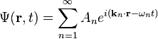
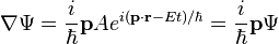
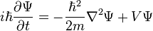
The form of the Schrödinger equation depends on the physical situation (see below for special cases). The most general form is the time-dependent Schrödinger equation, which gives a description of a system evolving with time:[5]:143Time-dependent Schrödinger equation (general)

.gif)
A wave function that satisfies the non-relativistic Schrödinger equation with V = 0. In other words, this corresponds to a particle traveling freely through empty space. The real part of the wave function is plotted here.
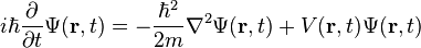
The most famous example is the non-relativistic Schrödinger equation for a single particle moving in an electric field (but not a magnetic field; see the Pauli equation):
Time-dependent Schrödinger equation
(single non-relativistic particle)
![i\hbar\frac{\partial}{\partial t} \Psi(\mathbf{r},t) = \left [ \frac{-\hbar^2}{2\mu}\nabla^2 + V(\mathbf{r},t)\right ] \Psi(\mathbf{r},t)](//upload.wikimedia.org/math/9/8/2/982d527d66c31874b0db94f603e3be2f.png)
![i\hbar\frac{\partial}{\partial t} \Psi(\mathbf{r},t) = \left [ \frac{-\hbar^2}{2\mu}\nabla^2 + V(\mathbf{r},t)\right ] \Psi(\mathbf{r},t)](http://upload.wikimedia.org/math/9/8/2/982d527d66c31874b0db94f603e3be2f.png)
Given the particular differential operators involved, this is a linear partial differential equation. It is also a diffusion equation, but unlike the heat equation, this one is also a wave equation given the imaginary unit present in the transient term.
The term "Schrödinger equation" can refer to both the general equation (first box above), or the specific nonrelativistic version (second box above and variations thereof). The general equation is indeed quite general, used throughout quantum mechanics, for everything from the Dirac equation to quantum field theory, by plugging in various complicated expressions for the Hamiltonian. The specific nonrelativistic version is a simplified approximation to reality, which is quite accurate in many situations, but very inaccurate in others (see relativistic quantum mechanics and relativistic quantum field theory).
To apply the Schrödinger equation, the Hamiltonian operator is set up for the system, accounting for the kinetic and potential energy of the particles constituting the system, then inserted into the Schrödinger equation. The resulting partial differential equation is solved for the wave function, which contains information about the system.
Time-independent equation

Each of these three rows is a wave function which satisfies the time-dependent Schrödinger equation for a harmonic oscillator. Left: The real part (blue) and imaginary part (red) of the wave function. Right: The probability distribution of finding the particle with this wave function at a given position. The top two rows are examples of stationary states, which correspond to standing waves. The bottom row is an example of a state which is not a stationary state. The right column illustrates why stationary states are called "stationary".
The time-independent Schrödinger equation predicts that wave functions can form standing waves, called stationary states (also called "orbitals", as in atomic orbitals or molecular orbitals). These states are important in their own right, and if the stationary states are classified and understood, then it becomes easier to solve the time-dependent Schrödinger equation for any state. The time-independent Schrödinger equation is the equation describing stationary states. (It is only used when the Hamiltonian itself is not dependent on time. In general, the wave function still has a time dependency.)
Time-independent Schrödinger equation (general)


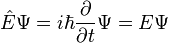
-
- When the Hamiltonian operator acts on a certain wave function Ψ, and the result is proportional to the same wave function Ψ, then Ψ is a stationary state, and the proportionality constant, E, is the energy of the state Ψ.
As before, the most famous manifestation is the non-relativistic Schrödinger equation for a single particle moving in an electric field (but not a magnetic field):
Time-independent Schrödinger equation (single non-relativistic particle)
![E \Psi(\mathbf{r}) = \left[ \frac{-\hbar^2}{2\mu}\nabla^2 + V(\mathbf{r}) \right] \Psi(\mathbf{r})](//upload.wikimedia.org/math/c/0/5/c059616c6d8ad2365b13734243343c8d.png)
![E \Psi(\mathbf{r}) = \left[ \frac{-\hbar^2}{2\mu}\nabla^2 + V(\mathbf{r}) \right] \Psi(\mathbf{r})](http://upload.wikimedia.org/math/c/0/5/c059616c6d8ad2365b13734243343c8d.png)
Implications
The Schrödinger equation, and its solutions, introduced a breakthrough in thinking about physics. Schrödinger's equation was the first of its type, and solutions led to consequences that were very unusual and unexpected for the time.Total, kinetic, and potential energy
The overall form of the equation is not unusual or unexpected as it uses the principle of the conservation of energy.The terms of the nonrelativistic Schrödinger equation can be interpreted as total energy of the system, equal to the system kinetic energy plus the system potential energy. In this respect, it is just the same as in classical physics.
Quantization
The Schrödinger equation predicts that if certain properties of a system are measured, the result may be quantized, meaning that only specific discrete values can occur. One example is energy quantization: the energy of an electron in an atom is always one of the quantized energy levels, a fact discovered via atomic spectroscopy. (Energy quantization is discussed below.) Another example is quantization of angular momentum. This was an assumption in the earlier Bohr model of the atom, but it is a prediction of the Schrödinger equation.Another result of the Schrödinger equation is that not every measurement gives a quantized result in quantum mechanics. For example, position, momentum, time, and (in some situations) energy can have any value across a continuous range.[6]:165–167
Measurement and uncertainty
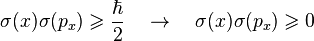
In classical mechanics, a particle has, at every moment, an exact position and an exact momentum. These values change deterministically as the particle moves according to Newton's laws. In quantum mechanics, particles do not have exactly determined properties, and when they are measured, the result is randomly drawn from a probability distribution. The Schrödinger equation predicts what the probability distributions are, but fundamentally cannot predict the exact result of each measurement.The Heisenberg uncertainty principle is the statement of the inherent measurement uncertainty in quantum mechanics. It states that the more precisely a particle's position is known, the less precisely its momentum is known, and vice versa.
The Schrödinger equation describes the (deterministic) evolution of the wave function of a particle. However, even if the wave function is known exactly, the result of a specific measurement on the wave function is uncertain.
Quantum tunneling

Quantum tunneling through a barrier. A particle coming from the left does not have enough energy to climb the barrier. However, it can sometimes "tunnel" to the other side.
In classical physics, when a ball is rolled slowly up a large hill, it will come to a stop and roll back, because it doesn't have enough energy to get over the top of the hill to the other side. However, the Schrödinger equation predicts that there is a small probability that the ball will get to the other side of the hill, even if it has too little energy to reach the top. This is called quantum tunneling. It is related to the distribution of energy: Although the ball's assumed position seems to be on one side of the hill, there is a chance of finding it on the other side.
Particles as waves

The nonrelativistic Schrödinger equation is a type of partial differential equation called a wave equation. Therefore it is often said particles can exhibit behavior usually attributed to waves. In most modern interpretations this description is reversed – the quantum state, i.e. wave, is the only genuine physical reality, and under the appropriate conditions it can show features of particle-like behavior.
Two-slit diffraction is a famous example of the strange behaviors that waves regularly display, that are not intuitively associated with particles. The overlapping waves from the two slits cancel each other out in some locations, and reinforce each other in other locations, causing a complex pattern to emerge. Intuitively, one would not expect this pattern from firing a single particle at the slits, because the particle should pass through one slit or the other, not a complex overlap of both.
However, since the Schrödinger equation is a wave equation, a single particle fired through a double-slit does show this same pattern (figure on right). Note: The experiment must be repeated many times for the complex pattern to emerge. The appearance of the pattern proves that each electron passes through both slits simultaneously.[7][8][9] Although this is counterintuitive, the prediction is correct; in particular, electron diffraction and neutron diffraction are well understood and widely used in science and engineering.
Related to diffraction, particles also display superposition and interference.
The superposition property allows the particle to be in a quantum superposition of two or more states with different classical properties at the same time. For example, a particle can have several different energies at the same time, and can be in several different locations at the same time. In the above example, a particle can pass through two slits at the same time. This superposition is still a single quantum state, as shown by the interference effects, even though that conflicts with classical intuition.
Interpretation of the wave function
The Schrödinger equation provides a way to calculate the wave function of a system and how it changes dynamically in time. However, the Schrödinger equation does not directly say what, exactly, the wave function is. Interpretations of quantum mechanics address questions such as what the relation is between the wave function, the underlying reality, and the results of experimental measurements.An important aspect is the relationship between the Schrödinger equation and wavefunction collapse. In the oldest Copenhagen interpretation, particles follow the Schrödinger equation except during wavefunction collapse, during which they behave entirely differently. The advent of quantum decoherence theory allowed alternative approaches (such as the Everett many-worlds interpretation and consistent histories), wherein the Schrödinger equation is always satisfied, and wavefunction collapse should be explained as a consequence of the Schrödinger equation.
Historical background and development
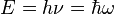
Following Max Planck's quantization of light (see black body radiation), Albert Einstein interpreted Planck's quanta to be photons, particles of light, and proposed that the energy of a photon is proportional to its frequency, one of the first signs of wave–particle duality. Since energy and momentum are related in the same way as frequency and wavenumber in special relativity, it followed that the momentum p of a photon is inversely proportional to its wavelength λ, or proportional to its wavenumber k.


In 1921, prior to de Broglie, Arthur C. Lunn at the University of Chicago had used the same argument based on the completion of the relativistic energy–momentum 4-vector to derive what we now call the de Broglie relation.[11]
Unlike de Broglie, Lunn went on to formulate the differential equation now known as the Schrödinger equation, and solve for its energy eigenvalues for the hydrogen atom. Unfortunately the paper was rejected by the Physical Review, as recounted by Kamen.[12]
Following up on de Broglie's ideas, physicist Peter Debye made an offhand comment that if particles behaved as waves, they should satisfy some sort of wave equation. Inspired by Debye's remark, Schrödinger decided to find a proper 3-dimensional wave equation for the electron. He was guided by William R. Hamilton's analogy between mechanics and optics, encoded in the observation that the zero-wavelength limit of optics resembles a mechanical system — the trajectories of light rays become sharp tracks that obey Fermat's principle, an analog of the principle of least action.[13] A modern version of his reasoning is reproduced below. The equation he found is:[14]
Schrödinger used the relativistic energy momentum relation to find what is now known as the Klein–Gordon equation in a Coulomb potential (in natural units):

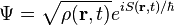
While at the cabin, Schrödinger decided that his earlier non-relativistic calculations were novel enough to publish, and decided to leave off the problem of relativistic corrections for the future. Despite the difficulties in solving the differential equation for hydrogen (he had sought help from his friend the mathematician Hermann Weyl[18]:3) Schrödinger showed that his non-relativistic version of the wave equation produced the correct spectral energies of hydrogen in a paper published in 1926.[18]:1[19] In the equation, Schrödinger computed the hydrogen spectral series by treating a hydrogen atom's electron as a wave Ψ(x, t), moving in a potential well V, created by the proton. This computation accurately reproduced the energy levels of the Bohr model. In a paper, Schrödinger himself explained this equation as follows:
| “ | The already ... mentioned psi-function.... is now the means for predicting probability of measurement results. In it is embodied the momentarily attained sum of theoretically based future expectation, somewhat as laid down in a catalog. | ” |
—Erwin Schrödinger[20]
|
||
This 1926 paper was enthusiastically endorsed by Einstein, who saw the matter-waves as an intuitive depiction of nature, as opposed to Heisenberg's matrix mechanics, which he considered overly formal.[21]
The Schrödinger equation details the behavior of Ψ but says nothing of its nature. Schrödinger tried to interpret it as a charge density in his fourth paper, but he was unsuccessful.[22]:219 In 1926, just a few days after Schrödinger's fourth and final paper was published, Max Born successfully interpreted Ψ as the probability amplitude, whose absolute square is equal to probability density.[22]:220 Schrödinger, though, always opposed a statistical or probabilistic approach, with its associated discontinuities—much like Einstein, who believed that quantum mechanics was a statistical approximation to an underlying deterministic theory— and never reconciled with the Copenhagen interpretation.[23]
Louis de Broglie in his later years proposed a real valued wave function connected to the complex wave function by a proportionality constant and developed the De Broglie–Bohm theory.
The wave equation for particles
The Schrödinger equation is a wave equation, since the solutions are functions which describe wave-like motions. Wave equations in physics can normally be derived from other physical laws – the wave equation for mechanical vibrations on strings and in matter can be derived from Newton's laws – where the wave function represents the displacement of matter, and electromagnetic waves from Maxwell's equations, where the wave functions are electric and magnetic fields. The basis for Schrödinger's equation, on the other hand, is the energy of the system and a separate postulate of quantum mechanics: the wave function is a description of the system.[24] The Schrödinger equation is therefore a new concept in itself; as Feynman put it:| “ | Where did we get that (equation) from? Nowhere. It is not possible to derive it from anything you know. It came out of the mind of Schrödinger. | ” |
—Richard Feynman[25]
|
||
Spherical harmonics are to the Schrödinger equation what the math of Henri Poincaré was to Einstein's theory of relativity: foundational.
The foundation of the equation is structured to be a linear differential equation based on classical energy conservation, and consistent with the De Broglie relations. The solution is the wave function ψ, which contains all the information that can be known about the system. In the Copenhagen interpretation, the modulus of ψ is related to the probability the particles are in some spatial configuration at some instant of time. Solving the equation for ψ can be used to predict how the particles will behave under the influence of the specified potential and with each other.
The Schrödinger equation was developed principally from the De Broglie hypothesis, a wave equation that would describe particles,[26] and can be constructed as shown informally in the following sections.[27] For a more rigorous description of Schrödinger's equation, see also.[28]
Consistency with energy conservation
The total energy E of a particle is the sum of kinetic energy T and potential energy V, this sum is also the frequent expression for the Hamiltonian H in classical mechanics:


Linearity
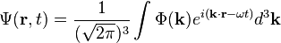
The simplest wavefunction is a plane wave of the form:
For discrete k the sum is a superposition of plane waves:
Consistency with the De Broglie relations

Diagrammatic summary of the quantities related to the wavefunction, as used in De broglie's hypothesis and development of the Schrödinger equation.[26]
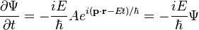
Einstein's light quanta hypothesis (1905) states that the energy E of a photon is proportional to the frequency ν (or angular frequency, ω = 2πν) of the corresponding quantum wavepacket of light:

Schrödinger's insight,[citation needed] late in 1925, was to express the phase of a plane wave as a complex phase factor using these relations:

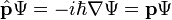
Substituting the energy and momentum operators into the classical energy conservation equation obtains the operator:


Wave and particle motion

Increasing levels of wavepacket localization, meaning
the particle has a more localized position.
the particle has a more localized position.

In the limit ħ → 0, the particle's position and momentum become known exactly. This is equivalent to the classical particle.
The limiting short-wavelength is equivalent to ħ tending to zero because this is limiting case of increasing the wave packet localization to the definite position of the particle (see images right). Using the Heisenberg uncertainty principle for position and momentum, the products of uncertainty in position and momentum become zero as ħ → 0:
The Schrödinger equation in its general form


Substituting
The implications are:
- The motion of a particle, described by a (short-wavelength) wave packet solution to the Schrödinger equation, is also described by the Hamilton–Jacobi equation of motion.
- The Schrödinger equation includes the wavefunction, so its wave packet solution implies the position of a (quantum) particle is fuzzily spread out in wave fronts. On the contrary, the Hamilton–Jacobi equation applies to a (classical) particle of definite position and momentum, instead the position and momentum at all times (the trajectory) are deterministic and can be simultaneously known.
Non-relativistic quantum mechanics
The quantum mechanics of particles without accounting for the effects of special relativity, for example particles propagating at speeds much less than light, is known as non-relativistic quantum mechanics. Following are several forms of Schrödinger's equation in this context for different situations: time independence and dependence, one and three spatial dimensions, and one and N particles.In actuality, the particles constituting the system do not have the numerical labels used in theory. The language of mathematics forces us to label the positions of particles one way or another, otherwise there would be confusion between symbols representing which variables are for which particle.[28]
Time independent
If the Hamiltonian is not an explicit function of time, the equation is separable into a product of spatial and temporal parts. In general, the wavefunction takes the form:
Substituting for ψ into the Schrödinger equation for the relevant number of particles in the relevant number of dimensions, solving by separation of variables implies the general solution of the time-dependent equation has the form:[14]


The energy eigenvalues from this equation form a discrete spectrum of values, so mathematically energy must be quantized. More specifically, the energy eigenstates form a basis – any wavefunction may be written as a sum over the discrete energy states or an integral over continuous energy states, or more generally as an integral over a measure. This is the spectral theorem in mathematics, and in a finite state space it is just a statement of the completeness of the eigenvectors of a Hermitian matrix.
One-dimensional examples
For a particle in one dimension, the Hamiltonian is:


Free particle
For no potential, V = 0, so the particle is free and the equation reads:[5]:151ff


Constant potential

Harmonic oscillator

A harmonic oscillator in classical mechanics (A–B) and quantum mechanics (C–H). In (A–B), a ball, attached to a spring, oscillates back and forth. (C–H) are six solutions to the Schrödinger Equation for this situation. The horizontal axis is position, the vertical axis is the real part (blue) or imaginary part (red) of the wavefunction. Stationary states, or energy eigenstates, which are solutions to the time-independent Schrödinger Equation, are shown in C,D,E,F, but not G or H.

There is a family of solutions – in the position basis they are

Three-dimensional examples
The extension from one dimension to three dimensions is straightforward, all position and momentum operators are replaced by their three-dimensional expressions and the partial derivative with respect to space is replaced by the gradient operator.The Hamiltonian for one particle in three dimensions is:


For N particles in three dimensions, the Hamiltonian is:


Following are examples where exact solutions are known.
Hydrogen atom
This form of the Schrödinger equation can be applied to the hydrogen atom:[24][26]

The wavefunction for hydrogen is a function of the electron's coordinates, and in fact can be separated into functions of each coordinate.[34] Usually this is done in spherical polar coordinates:

 are spherical harmonics of degree ℓ and order m. This is the only atom for which the Schrödinger equation has been solved for exactly. Multi-electron atoms require approximative methods. The family of solutions are:[35]
![\psi_{n\ell m}(r,\theta,\phi) = \sqrt {{\left ( \frac{2}{n a_0} \right )}^3\frac{(n-\ell-1)!}{2n[(n+\ell)!]} } e^{- r/na_0} \left(\frac{2r}{na_0}\right)^{\ell} L_{n-\ell-1}^{2\ell+1}\left(\frac{2r}{na_0}\right) \cdot Y_{\ell}^{m}(\theta, \phi )](http://upload.wikimedia.org/math/4/5/c/45cf853209a6e1ab610563d737c08edd.png)
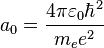 is the Bohr radius,
 are the generalized Laguerre polynomials of degree n − ℓ − 1.
- n, ℓ, m are the principal, azimuthal, and magnetic quantum numbers respectively: which take the values:
 is the
  are the
Two-electron atoms or ions
The equation for any two-electron system, such as the neutral helium atom (He, Z = 2), the negative hydrogen ion (H−, Z = 1), or the positive lithium ion (Li+, Z = 3) is:[27]![E\psi = -\hbar^2\left[\frac{1}{2\mu}\left(\nabla_1^2 +\nabla_2^2 \right) + \frac{1}{M}\nabla_1\cdot\nabla_2\right] \psi + \frac{e^2}{4\pi\epsilon_0}\left[ \frac{1}{r_{12}} -Z\left( \frac{1}{r_1}+\frac{1}{r_2} \right) \right] \psi](http://upload.wikimedia.org/math/3/5/1/35130911dffc1f9088118d1edd21ab1f.png)


The cross-term of two laplacians

Time dependent
This is the equation of motion for the quantum state. In the most general form, it is written:[5]:143ff
For one particle in one dimension, the Hamiltonian


Solution methods
General techniques:
|
Methods for special cases:
|
Properties
The Schrödinger equation has the following properties: some are useful, but there are shortcomings. Ultimately, these properties arise from the Hamiltonian used, and solutions to the equation.Linearity
In the development above, the Schrödinger equation was made to be linear for generality, though this has other implications. If two wave functions ψ1 and ψ2 are solutions, then so is any linear combination of the two:


Real energy eigenstates
For the time-independent equation, an additional feature of linearity follows: if two wave functions ψ1 and ψ2 are solutions to the time-independent equation with the same energy E, then so is any linear combination:
In an arbitrary potential, if a wave function ψ solves the time-independent equation, so does its complex conjugate, denoted ψ*. By taking linear combinations, the real and imaginary parts of ψ are each solutions. If there is no degeneracy they can only differ by a factor.
In the time-dependent equation, complex conjugate waves move in opposite directions. If Ψ(x, t) is one solution, then so is Ψ(x, –t). The symmetry of complex conjugation is called time-reversal symmetry.
Space and time derivatives

The Schrödinger equation is first order in time and second in space, which describes the time evolution of a quantum state (meaning it determines the future amplitude from the present).
Explicitly for one particle in 3-dimensional Cartesian coordinates – the equation is


As the first order derivatives are arbitrary, the wavefunction can be a continuously differentiable function of space, since at any boundary the gradient of the wavefunction can be matched.
On the contrary, wave equations in physics are usually second order in time, notable are the family of classical wave equations and the quantum Klein–Gordon equation.
Local conservation of probability
The Schrödinger equation is consistent with probability conservation. Multiplying the Schrödinger equation on the right by the complex conjugate wavefunction, and multiplying the wavefunction to the left of the complex conjugate of the Schrödinger equation, and subtracting, gives the continuity equation for probability:[36]
Hence predictions from the Schrödinger equation do not violate probability conservation.
Positive energy
If the potential is bounded from below, meaning there is a minimum value of potential energy, the eigenfunctions of the Schrödinger equation have energy which is also bounded from below. This can be seen most easily by using the variational principle, as follows. (See also below).For any linear operator  bounded from below, the eigenvector with the smallest eigenvalue is the vector ψ that minimizes the quantity

![\langle \psi|\hat{H}|\psi\rangle = \int \psi^*(\mathbf{r}) \left[ - \frac{\hbar^2}{2m} \nabla^2\psi(\mathbf{r}) + V(\mathbf{r})\psi(\mathbf{r})\right] d^3\mathbf{r} = \int \left[ \frac{\hbar^2}{2m}|\nabla\psi|^2 + V(\mathbf{r}) |\psi|^2 \right] d^3\mathbf{r} = \langle \hat{H}\rangle](http://upload.wikimedia.org/math/6/a/b/6ab88bfe085f73c8f8ed867b24f7bded.png)
For potentials which are bounded below and are not infinite over a region, there is a ground state which minimizes the integral above. This lowest energy wavefunction is real and positive definite – meaning the wavefunction can increase and decrease, but is positive for all positions. It physically cannot be negative: if it were, smoothing out the bends at the sign change (to minimize the wavefunction) rapidly reduces the gradient contribution to the integral and hence the kinetic energy, while the potential energy changes linearly and less quickly. The kinetic and potential energy are both changing at different rates, so the total energy is not constant, which can't happen (conservation).
The solutions are consistent with Schrödinger equation if this wavefunction is positive definite.
The lack of sign changes also shows that the ground state is nondegenerate, since if there were two ground states with common energy E, not proportional to each other, there would be a linear combination of the two that would also be a ground state resulting in a zero solution.
Analytic continuation to diffusion
The above properties (positive definiteness of energy) allow the analytic continuation of the Schrödinger equation to be identified as a stochastic process. This can be interpreted as the Huygens–Fresnel principle applied to De Broglie waves; the spreading wavefronts are diffusive probability amplitudes.[36]For a free particle (not subject to a potential) in a random walk, substituting τ = it into the time-dependent Schrödinger equation gives:[37]

Relativistic quantum mechanics
Relativistic quantum mechanics is obtained where quantum mechanics and special relativity simultaneously apply. In general, one wishes to build relativistic wave equations from the relativistic energy–momentum relation
The Klein–Gordon equation was the first such equation to be obtained, even before the non-relativistic one, and applies to massive spinless particles. The Dirac equation arose from taking the "square root" of the Klein–Gordon equation by factorizing the entire relativistic wave operator into a product of two operators – one of these is the operator for the entire Dirac equation.
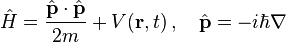
The general form of the Schrödinger equation remains true in relativity, but the Hamiltonian is less obvious. For example, the Dirac Hamiltonian for a particle of mass m and electric charge q in an electromagnetic field (described by the electromagnetic potentials φ and A) is:
![\hat{H}_{\text{Dirac}}= \gamma^0 \left[c \boldsymbol{\gamma}\cdot\left(\hat{\mathbf{p}} - q \mathbf{A}\right) + mc^2 + \gamma^0q \phi \right]\,,](http://upload.wikimedia.org/math/3/8/6/38600e55729f2e388fccd2ba301c7f18.png)
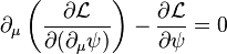
For the Klein–Gordon equation, the general form of the Schrödinger equation is inconvenient to use, and in practice the Hamiltonian is not expressed in an analogous way to the Dirac Hamiltonian. The equations for relativistic quantum fields can be obtained in other ways, such as starting from a Lagrangian density and using the Euler-Lagrange equations for fields, or use the representation theory of the Lorentz group in which certain representations can be used to fix the equation for a free particle of given spin (and mass).
In general, the Hamiltonian to be substituted in the general Schrödinger equation is not just a function of the position and momentum operators (and possibly time), but also of spin matrices. Also, the solutions to a relativistic wave equation, for a massive particle of spin s, are complex-valued 2(2s + 1)-component spinor fields.


 stands for the four real numbers which give the time and position in three dimensions of the point labeled A.

 are
are  a
a  , called "psi-bar", is sometimes referred to as the
  is the
 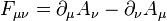 is the


 , will give a final state
  in such a way to have

![U=T\exp\left[-\frac{i}{\hbar}\int_{t_0}^tdt'V(t')\right]](http://upload.wikimedia.org/math/f/f/c/ffce1a89c334d137bda73d0ccba5aa1a.png)
 , since these internal ("virtual") particles are not constrained to any specific energy–momentum – even that usually required by special relativity (see


