From Wikipedia, the free encyclopedia
This article is about a simplified presentation of electromagnetism, incorporating special relativity. For a more general article on the relationship between special relativity and electromagnetism, see Classical electromagnetism and special relativity. For a more rigorous discussion, see Covariant formulation of classical electromagnetism.
Relativistic electromagnetism is a modern teaching strategy for developing electromagnetic field theory from Coulomb's law and Lorentz transformations. Though Coulomb's law expresses action at a distance, it is an easily understood electric force principle. The more sophisticated view of electromagnetism expressed by electromagnetic fields in spacetime can be approached by applying spacetime symmetries. In certain special configurations it is possible to exhibit magnetic effects due to relative charge density in various simultaneous hyperplanes. This approach to physics education and the education and training of electrical and electronics engineers can be seen in the Encyclopædia Britannica (1956), The Feynman Lectures on Physics (1964), Edward M. Purcell (1965), Jack R. Tessman (1966), W.G.V. Rosser (1968), Anthony French (1968), and Dale R. Corson & Paul Lorrain (1970). This approach provides some preparation for understanding of magnetic forces involved in the Biot–Savart law, Ampère's law, and Maxwell's equations.In 1912 Leigh Page expressed the aspiration of relativistic electromagnetism:[1]
- If the principle of relativity had been enunciated before the date of Oersted’s discovery, the fundamental relations of electrodynamics could have been predicted on theoretical grounds as a direct consequence of the fundamental laws of electrostatics, extended so as to apply to charges relatively in motion as well as charges relatively at rest.
Einstein's motivation
In 1953 Albert Einstein wrote to the Cleveland Physics Society on the occasion of a commemoration of the Michelson–Morley experiment. In that letter he wrote:[2]- What led me more or less directly to the special theory of relativity was the conviction that the electromotive force acting on a body in motion in a magnetic field was nothing else but an electric field.
Introduction
Purcell argued that the question of an electric field in one inertial frame of reference, and how it looks from a different reference frame moving with respect to the first, is crucial to understand fields created by moving sources. In the special case, the sources that create the field are at rest with respect to one of the reference frames. Given the electric field in the frame where the sources are at rest, Purcell asked: what is the electric field in some other frame?He stated that the fundamental assumption is that, knowing the electric field at some point (in space and time) in the rest frame of the sources, and knowing the relative velocity of the two frames provided all the information needed to calculate the electric field at the same point in the other frame. In other words, the electric field in the other frame does not depend on the particular distribution of the source charges, only on the local value of the electric field in the first frame at that point. He assumed that the electric field is a complete representation of the influence of the far-away charges.
Alternatively, introductory treatments of magnetism introduce the Biot–Savart law, which describes the magnetic field associated with an electric current. An observer at rest with respect to a system of static, free charges will see no magnetic field. However, a moving observer looking at the same set of charges does perceive a current, and thus a magnetic field.
Uniform electric field — simple analysis

Figure 1: Two oppositely charged plates produce uniform electric field even when moving. The electric field is shown as 'flowing' from top to bottom plate. The Gaussian pill box (at rest) can be used to find the strength of the field.
Consider the very simple situation of a charged parallel-plate capacitor, whose electric field (in its rest frame) is uniform (neglecting edge effects) between the plates and zero outside.
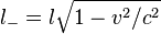
To calculate the electric field of this charge distribution in a reference frame where it is in motion, suppose that the motion is in a direction parallel to the plates as shown in figure 1. The plates will then be shorter by a factor of:


More rigorous analysis

Figure 2a: The electric field lines are shown flowing outward from the positive plate

Figure 2b: The electric field lines flow inward toward the negative plate
Consider the electric field of a single, infinite plate of positive charge, moving parallel to itself. The field must be uniform both above and below the plate, since it is uniform in its rest frame. We also assume that knowing the field in one frame is sufficient for calculating it in the other frame.
The plate however could have a non zero component of electric field in the direction of motion as in Fig 2a. Even in this case, the field of the infinite plane of negative charge must be equal and opposite to that of the positive plate (as in Fig 2b), since the combination of plates is neutral and cannot therefore produce any net fields. When the plates are separated, the horizontal components still cancel, and the resultant is a uniform vertical field as shown in Fig 1.
If Gauss's law is applied to pillbox as shown in Fig 1, it can be shown that the magnitude of the electric field between the plates is given by:

 represents the surface charge density of the positive plate. Since the plates are contracted in length by the factor


These transformation equations only apply if the source of the field is at rest in the unprimed frame.
The field of a moving point charge[edit]

Figure 3: A point charge at rest, surrounded by an imaginary sphere.

Figure 4: A view of the electric field of a point charge moving at constant velocity.
A very important application of the electric field transformation equations is to the field of a single point charge moving with constant velocity. In its rest frame, the electric field of a positive point charge has the same strength in all directions and points directly away from the charge. In some other reference frame the field will appear differently.
In applying the transformation equations to a nonuniform electric field, it is important to record not only the value of the field, but also at what point in space it has this value.
In the rest frame of the particle, the point charge can be imagined to be surrounded by a spherical shell which is also at rest. In our reference frame, however, both the particle and its sphere are moving. Length contraction therefore states that the sphere is deformed into an oblate spheroid, as shown in cross section in Fig 4.
Consider the value of the electric field at any point on the surface of the sphere. Let x and y be the components of the displacement (in the rest frame of the charge), from the charge to a point on the sphere, measured parallel and perpendicular to the direction of motion as shown in the figure. Because the field in the rest frame of the charge points directly away from the charge, its components are in the same ratio as the components of the displacement:


However, according to the above results, the y component of the field is enhanced by a similar factor:

The origin of magnetic forces

Figure 5, lab frame: A horizontal wire carrying a current, represented by evenly spaced positive charges moving to the right whilst an equal number of negative charges remain at rest, with a positively charged particle outside the wire and traveling in a direction parallel to the current.
In the simple model of events in a wire stretched out horizontally, a current can be represented by the evenly spaced positive charges, moving to the right, whilst an equal number of negative charges remain at rest. If the wire is electrostatically neutral, the distance between adjacent positive charges must be the same as the distance between adjacent negative charges.
Assume that in our 'lab frame' (Figure 5), we have a positive test charge, Q, outside the wire, traveling parallel to the current, at the speed, v, which is equal to the speed of the moving charges in the wire. It should experience a magnetic force, which can be easily confirmed by experiment.

Figure 6, test charge frame: The same situation as in fig. 5, but viewed from the reference frame in which positive charges are at rest. The negative charges flow to the left. The distance between the negative charges is length-contracted relative to the lab frame, while the distance between the positive charges is expanded, so the wire carries a net negative charge.
Inside 'test charge frame'(Fig. 6), the only possible force is the electrostatic force Fe = Q * E because, although the magnetic field is the same, the test charge is at rest and, therefore, cannot feel it. In this frame, the negative charge density has Lorentz-contracted with respect to what we had in lab frame because of the increased speed. This means that spacing between charges has reduced by the Lorentz factor with respect to the lab frame spacing, l:

For
 , we can concretely compute both,[3] the magnetic force sensed in the lab frame

 , resulting electrostatic force
 .
.The lesson is that observers in different frames of reference see the same phenomena but disagree on their reasons.
If the currents are in opposite directions, consider the charge moving to the left. No charges are now at rest in the reference frame of the test charge. The negative charges are moving with speed v in the test charge frame so their spacing is again:


One may think that the picture, presented here, is artificial because electrons, which accelerated in fact, must condense in the lab frame, making the wire charged. Naturally, however, all electrons feel the same accelerating force and, therefore, identically to the Bell's spaceships, the distance between them does not change in the lab frame (i.e. expands in their proper moving frame). Rigid bodies, like trains, don't expand however in their proper frame, and, therefore, really contract, when observed from the stationary frame.
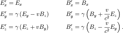
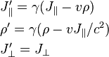
 while the fields perpendicular to v are denoted as
  . In these two frames moving at relative velocity v, the E-fields and B-fields are related by:


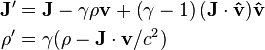
 is the parallel component of A to the direction of relative velocity between frames v, and
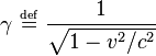
  is the perpendicular component. These transparently resemble the characteristic form of other Lorentz transformations (like time-position and energy-momentum), while the transformations of E and B above are slightly more complicated. The components can be collected together as:


 ,
,


 is the contravariant
  .
.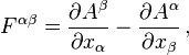


 is the

