Coral reef

From Wikipedia, the free encyclopedia

Marine habitats
Biodiversity of a coral reef
Littoral zone Intertidal zone Estuaries Kelp forests Coral reefs Ocean banks Continental shelf Neritic zone Straits Pelagic zone Oceanic zone Seamounts Hydrothermal vents Cold seeps Demersal zone Benthic zone
v t e

Coral reefs are diverse underwater ecosystems held together by calcium carbonate structures secreted by corals. Coral reefs are built by colonies of tiny animals found in marine water that contain few nutrients. Most coral reefs are built from stony corals, which in turn consist of polyps that cluster in groups. The polyps belong to a group of animals known as Cnidaria, which also includes sea anemones and jellyfish. Unlike sea anemones, corals secrete hard carbonate exoskeletons which support and protect the coral polyps. Most reefs grow best in warm, shallow, clear, sunny and agitated water.

Often called "rainforests of the sea", shallow coral reefs form some of the most diverse ecosystems on Earth. They occupy less than 0.1% of the world's ocean surface, about half the area of France, yet they provide a home for at least 25% of all marine species,^[1][2][3][4] including fish, mollusks, worms, crustaceans, echinoderms, sponges, tunicates and other cnidarians.^[5] Paradoxically, coral reefs flourish even though they are surrounded by ocean waters that provide few nutrients. They are most commonly found at shallow depths in tropical waters, but deep water and cold water corals also exist on smaller scales in other areas.

Coral reefs deliver ecosystem services to tourism, fisheries and shoreline protection. The annual global economic value of coral reefs is estimated between US$30–375 billion.^[6][7] However, coral reefs are fragile ecosystems, partly because they are very sensitive to water temperature. They are under threat from climate change, oceanic acidification, blast fishing, cyanide fishing for aquarium fish, sunscreen use,^[8] overuse of reef resources, and harmful land-use practices, including urban and agricultural runoff and water pollution, which can harm reefs by encouraging excess algal growth.^[9][10][11]

Formation

Most of the coral reefs we can see today were formed after the last glacial period when melting ice caused the sea level to rise and flood the continental shelves. This means that most modern coral reefs are less than 10,000 years old. As communities established themselves on the shelves, the reefs grew upwards, pacing rising sea levels. Reefs that rose too slowly could become drowned reefs. They are covered by so much water that there was insufficient light.^[12] Coral reefs are found in the deep sea away from continental shelves, around oceanic islands and as atolls. The vast majority of these islands are volcanic in origin. The few exceptions have tectonic origins where plate movements have lifted the deep ocean floor on the surface.
In 1842 in his first monograph, The Structure and Distribution of Coral Reefs,^[13] Charles Darwin set out his theory of the formation of atoll reefs, an idea he conceived during the voyage of the Beagle. He theorized uplift and subsidence of the Earth's crust under the oceans formed the atolls.^[14] Darwin’s theory sets out a sequence of three stages in atoll formation. It starts with a fringing reef forming around an extinct volcanic island as the island and ocean floor subsides. As the subsidence continues, the fringing reef becomes a barrier reef, and ultimately an atoll reef.

• 

  Darwin’s theory starts with a volcanic island which becomes extinct
  
• 

  As the island and ocean floor subside, coral growth builds a fringing reef, often including a shallow lagoon between the land and the main reef.
  
• 

  As the subsidence continues, the fringing reef becomes a larger barrier reef further from the shore with a bigger and deeper lagoon inside.
  
• 

  Ultimately, the island sinks below the sea, and the barrier reef becomes an atoll enclosing an open lagoon.
  

Darwin predicted that underneath each lagoon would be a bed rock base, the remains of the original volcano. Subsequent drilling proved this correct. Darwin's theory followed from his understanding that coral polyps thrive in the clean seas of the tropics where the water is agitated, but can only live within a limited depth range, starting just below low tide. Where the level of the underlying earth allows, the corals grow around the coast to form what he called fringing reefs, and can eventually grow out from the shore to become a barrier reef.

A fringing reef can take ten thousand years to form, and an atoll can take up to 30 million years.^[15]

Where the bottom is rising, fringing reefs can grow around the coast, but coral raised above sea level dies and becomes white limestone. If the land subsides slowly, the fringing reefs keep pace by growing upwards on a base of older, dead coral, forming a barrier reef enclosing a lagoon between the reef and the land. A barrier reef can encircle an island, and once the island sinks below sea level a roughly circular atoll of growing coral continues to keep up with the sea level, forming a central lagoon. Barrier reefs and atolls do not usually form complete circles, but are broken in places by storms. Like sea level rise, a rapidly subsiding bottom can overwhelm coral growth, killing the coral polyps and the reef, due to what is called coral drowning.^[16] Corals that rely on zooxanthellae can drown when the water becomes too deep for their symbionts to adequately photosynthesize, due to decreased light exposure.^[17]

The two main variables determining the geomorphology, or shape, of coral reefs are the nature of the underlying substrate on which they rest, and the history of the change in sea level relative to that substrate.

The approximately 20,000-year-old Great Barrier Reef offers an example of how coral reefs formed on continental shelves. Sea level was then 120 m (390 ft) lower than in the 21st century.^[18][19] As sea level rose, the water and the corals encroached on what had been hills of the Australian coastal plain. By 13,000 years ago, sea level had risen to 60 m (200 ft) lower than at present, and many hills of the coastal plains had become continental islands. As the sea level rise continued, water topped most of the continental islands. The corals could then overgrow the hills, forming the present cays and reefs. Sea level on the Great Barrier Reef has not changed significantly in the last 6,000 years,^[19] and the age of the modern living reef structure is estimated to be between 6,000 and 8,000 years.^[20] Although the Great Barrier Reef formed along a continental shelf, and not around a volcanic island, Darwin's principles apply. Development stopped at the barrier reef stage, since Australia is not about to submerge. It formed the world's largest barrier reef, 300–1,000 m (980–3,280 ft) from shore, stretching for 2,000 km (1,200 mi).^[21]

Healthy tropical coral reefs grow horizontally from 1 to 3 cm (0.39 to 1.18 in) per year, and grow vertically anywhere from 1 to 25 cm (0.39 to 9.84 in) per year; however, they grow only at depths shallower than 150 m (490 ft) because of their need for sunlight, and cannot grow above sea level.^[22]

Materials

As the name implies, the bulk of coral reefs is made up of coral skeletons from mostly intact coral colonies. As other chemical elements present in corals become incorporated into the calcium carbonate deposits, aragonite is formed. However, shell fragments and the remains of calcareous algae such as the green-segmented genus Halimeda can add to the reef's ability to withstand damage from storms and other threats. Such mixtures are visible in structures such as Eniwetok Atoll.^[23]

Types

The three principal reef types are:

• Fringing reef – directly attached to a shore, or borders it with an intervening shallow channel or lagoon
• Barrier reef – reef separated from a mainland or island shore by a deep channel or lagoon
• Atoll reef – more or less circular or continuous barrier reef extends all the way around a lagoon without a central island

A small atoll in the Maldives

Inhabited cay in the Maldives

Other reef types or variants are:

• Patch reef – common, isolated, comparatively small reef outcrop, usually within a lagoon or embayment, often circular and surrounded by sand or seagrass
• Apron reef – short reef resembling a fringing reef, but more sloped; extending out and downward from a point or peninsular shore
• Bank reef – linear or semicircular shaped-outline, larger than a patch reef
• Ribbon reef – long, narrow, possibly winding reef, usually associated with an atoll lagoon
• Table reef – isolated reef, approaching an atoll type, but without a lagoon
• Habili – reef specific to the Red Sea; does not reach the surface near enough to cause visible surf; may be a hazard to ships (from the Arabic for "unborn")
• Microatoll – community of species of corals; vertical growth limited by average tidal height; growth morphologies offer a low-resolution record of patterns of sea level change; fossilized remains can be dated using radioactive carbon dating and have been used to reconstruct Holocene sea levels^[24]
• Cays – small, low-elevation, sandy islands formed on the surface of coral reefs from eroded material that piles up, forming an area above sea level; can be stabilized by plants to become habitable; occur in tropical environments throughout the Pacific, Atlantic and Indian Oceans (including the Caribbean and on the Great Barrier Reef and Belize Barrier Reef), where they provide habitable and agricultural land
• Seamount or guyot – formed when a coral reef on a volcanic island subsides; tops of seamounts are rounded and guyots are flat; flat tops of guyots, or tablemounts, are due to erosion by waves, winds, and atmospheric processes

Zones

The three major zones of a coral reef: the fore reef, reef crest, and the back reef

Coral reef ecosystems contain distinct zones that represent different kinds of habitats. Usually, three major zones are recognized: the fore reef, reef crest, and the back reef (frequently referred to as the reef lagoon).

All three zones are physically and ecologically interconnected. Reef life and oceanic processes create opportunities for exchange of seawater, sediments, nutrients, and marine life among one another.

Thus, they are integrated components of the coral reef ecosystem, each playing a role in the support of the reefs' abundant and diverse fish assemblages.

Most coral reefs exist in shallow waters less than 50 m deep. Some inhabit tropical continental shelves where cool, nutrient rich upwelling does not occur, such as Great Barrier Reef. Others are found in the deep ocean surrounding islands or as atolls, such as in the Maldives. The reefs surrounding islands form when islands subside into the ocean, and atolls form when an island subsides below the surface of the sea.

Alternatively, Moyle and Cech distinguish six zones, though most reefs possess only some of the zones.^[25]

Water in the reef surface zone is often agitated. This diagram represents a reef on a continental shelf. The water waves at the left travel over the off-reef floor until they encounter the reef slope or fore reef. Then the waves pass over the shallow reef crest. When a wave enters shallow water it shoals, that is, it slows down and the wave height increases.

The reef surface is the shallowest part of the reef. It is subject to the surge and the rise and fall of tides. When waves pass over shallow areas, they shoal, as shown in the diagram at the right. This means the water is often agitated. These are the precise condition under which corals flourish. Shallowness means there is plenty of light for photosynthesis by the symbiotic zooxanthellae, and agitated water promotes the ability of coral to feed on plankton. However, other organisms must be able to withstand the robust conditions to flourish in this zone.

The off-reef floor is the shallow sea floor surrounding a reef. This zone occurs by reefs on continental shelves. Reefs around tropical islands and atolls drop abruptly to great depths, and do not have a floor. Usually sandy, the floor often supports seagrass meadows which are important foraging areas for reef fish.

The reef drop-off is, for its first 50 m, habitat for many reef fish who find shelter on the cliff face and plankton in the water nearby. The drop-off zone applies mainly to the reefs surrounding oceanic islands and atolls.

The reef face is the zone above the reef floor or the reef drop-off. This zone is often the most diverse area of the reef. Coral and calcareous algae growths provide complex habitats and areas which offer protection, such as cracks and crevices. Invertebrates and epiphytic algae provide much of the food for other organisms.^[25] A common feature on this forereef zone is spur and groove formations which serve to transport sediment downslope.

The reef flat is the sandy-bottomed flat, which can be behind the main reef, containing chunks of coral. This zone may border a lagoon and serve as a protective area, or it may lie between the reef and the shore, and in this case is a flat, rocky area. Fishes tend to prefer living in that flat, rocky area, compared to any other zone, when it is present.^[25]

The reef lagoon is an entirely enclosed region, which creates an area less affected by wave action that often contains small reef patches.^[25]

However, the "topography of coral reefs is constantly changing. Each reef is made up of irregular patches of algae, sessile invertebrates, and bare rock and sand. The size, shape and relative abundance of these patches changes from year to year in response to the various factors that favor one type of patch over another. Growing coral, for example, produces constant change in the fine structure of reefs. On a larger scale, tropical storms may knock out large sections of reef and cause boulders on sandy areas to move."^[26]

Locations

Locations of coral reefs

Boundary for 20 °C isotherms. Most corals live within this boundary. Note the cooler waters caused by upwelling on the southwest coast of Africa and off the coast of Peru.

This map shows areas of upwelling in red. Coral reefs are not found in coastal areas where colder and nutrient-rich upwellings occur.

Marine biodiversity of Raja Ampat Islands, Indonesia. It is estimated that about 75% of world coral reef population are in the Raja Ampat Islands

Coral reefs are estimated to cover 284,300 km² (109,800 sq mi),^[27] just under 0.1% of the oceans' surface area. The Indo-Pacific region (including the Red Sea, Indian Ocean, Southeast Asia and the Pacific) account for 91.9% of this total. Southeast Asia accounts for 32.3% of that figure, while the Pacific including Australia accounts for 40.8%. Atlantic and Caribbean coral reefs account for 7.6%.^[2]

Although corals exist both in temperate and tropical waters, shallow-water reefs form only in a zone extending from approximately 30° N to 30° S of the equator. Tropical corals do not grow at depths of over 50 meters (160 ft). The optimum temperature for most coral reefs is 26–27 °C (79–81 °F), and few reefs exist in waters below 18 °C (64 °F).^[28] However, reefs in the Persian Gulf have adapted to temperatures of 13 °C (55 °F) in winter and 38 °C (100 °F) in summer.^[29] There are 37 species of scleractinian corals identified in such harsh environment around Larak Island.^[30]

Deep-water coral can exist at greater depths and colder temperatures at much higher latitudes, as far north as Norway.^[31] Although deep water corals can form reefs, very little is known about them.

Coral reefs are rare along the west coasts of the Americas and Africa, due primarily to upwelling and strong cold coastal currents that reduce water temperatures in these areas (respectively the Peru, Benguela and Canary streams).^[32] Corals are seldom found along the coastline of South Asia—from the eastern tip of India (Chennai) to the Bangladesh and Myanmar borders^[2]—as well as along the coasts of northeastern South America and Bangladesh, due to the freshwater release from the Amazon and Ganges Rivers respectively.

• The Great Barrier Reef—largest, comprising over 2,900 individual reefs and 900 islands stretching for over 2,600 kilometers (1,600 mi) off Queensland, Australia
• The Mesoamerican Barrier Reef System—second largest, stretching 1,000 kilometers (620 mi) from Isla Contoy at the tip of the Yucatán Peninsula down to the Bay Islands of Honduras
• The New Caledonia Barrier Reef—second longest double barrier reef, covering 1,500 kilometers (930 mi)
• The Andros, Bahamas Barrier Reef—third largest, following the east coast of Andros Island, Bahamas, between Andros and Nassau
• The Red Sea—includes 6000-year-old fringing reefs located around a 2,000 km (1,240 mi) coastline
• The Florida Reef Tract—largest continental US reef and the third largest coral barrier reef system in the world, extends from Soldier Key, located in Biscayne Bay, to the Dry Tortugas in the Gulf of Mexico^[33]
• Pulley Ridge—deepest photosynthetic coral reef, Florida
• Numerous reefs scattered over the Maldives
• The Philippines coral reef area, the second largest in Southeast Asia, is estimated at 26,000 square kilometers and holds an extraordinary diversity of species. Scientists have identified 915 reef fish species and more than 400 scleractinian coral species, 12 of which are endemic.
• The Raja Ampat Islands in Indonesia's West Papua province offer the highest known marine diversity.^[34]
• Bermuda is known for its northernmost coral reef system, located at 32.4° N and 64.8° W. The presence of coral reefs at this high latitude is due to the proximity of the Gulf Stream. Bermuda has a fairly consistent diversity of coral species, representing a subset of those found in the greater Caribbean.^[35]
• The world's northernmost individual coral reef so far discovered is located within a bay of Japan's Tsushima Island in the Korea Strait.^[36]
• The world's southernmost coral reef is at Lord Howe Island, in the Pacific Ocean off the east coast of Australia.

Biology

Anatomy of a coral polyp

Alive corals are colonies of small animals embedded in calcium carbonate shells. It is a mistake to think of coral as plants or rocks. Coral heads consist of accumulations of individual animals called polyps, arranged in diverse shapes.^[37] Polyps are usually tiny, but they can range in size from a pinhead to 12 inches (30 cm) across.

Reef-building or hermatypic corals live only in the photic zone (above 50 m), the depth to which sufficient sunlight penetrates the water, allowing photosynthesis to occur. Coral polyps do not photosynthesize, but have a symbiotic relationship with microscopic algae of the genus Symbiodinium, commonly referred to as zooxanthellae. These organisms live within the tissues of polyps and provide organic nutrients that nourish the polyp. Because of this relationship, coral reefs grow much faster in clear water, which admits more sunlight. Without their symbionts, coral growth would be too slow to form significant reef structures. Corals get up to 90% of their nutrients from their symbionts.^[38]

Reefs grow as polyps and other organisms deposit calcium carbonate,^[39][40] the basis of coral, as a skeletal structure beneath and around themselves, pushing the coral head's top upwards and outwards.^[41] Waves, grazing fish (such as parrotfish), sea urchins, sponges, and other forces and organisms act as bioeroders, breaking down coral skeletons into fragments that settle into spaces in the reef structure or form sandy bottoms in associated reef lagoons. Many other organisms living in the reef community contribute skeletal calcium carbonate in the same manner.^[42] Coralline algae are important contributors to reef structure in those parts of the reef subjected to the greatest forces by waves (such as the reef front facing the open ocean). These algae strengthen the reef structure by depositing limestone in sheets over the reef surface.

Typical shapes for coral species are wrinkled brains, cabbages, table tops, antlers, wire strands and pillars. These shapes can depend on the life history of the coral, like light exposure and wave action,^[43] and events such as breakages.^[44]

Table coral

Close up of polyps are arrayed on a coral, waving their tentacles. There can be thousands of polyps on a single coral branch.

Corals reproduce both sexually and asexually. An individual polyp uses both reproductive modes within its lifetime. Corals reproduce sexually by either internal or external fertilization. The reproductive cells are found on the mesenteries, membranes that radiate inward from the layer of tissue that lines the stomach cavity. Some mature adult corals are hermaphroditic; others are exclusively male or female. A few species change sex as they grow.

Internally fertilized eggs develop in the polyp for a period ranging from days to weeks. Subsequent development produces a tiny larva, known as a planula. Externally fertilized eggs develop during synchronized spawning. Polyps release eggs and sperm into the water en masse, simultaneously. Eggs disperse over a large area. The timing of spawning depends on time of year, water temperature, and tidal and lunar cycles. Spawning is most successful when there is little variation between high and low tide. The less water movement, the better the chance for fertilization. Ideal timing occurs in the spring. Release of eggs or planula usually occurs at night, and is sometimes in phase with the lunar cycle (three to six days after a full moon). The period from release to settlement lasts only a few days, but some planulae can survive afloat for several weeks. They are vulnerable to predation and environmental conditions. The lucky few planulae which successfully attach to substrate next confront competition for food and space.^{[citation needed]}

There are eight clades of Symbiodinium phylotypes. Most research has been completed on the Symbiodinium clades A–D. Each one of the eight contributes their own benefits as well as less compatible attributes to the survival of their coral hosts. Each photosynthetic organism has a specific level of sensitivity to photodamage of compounds needed for survival, such as proteins. Rates of regeneration and replication determine the organism's ability to survive. Phylotype A is found more in the shallow regions of marine waters. It is able to produce mycosporine-like amino acids that are UV resistant, using a derivative of glycerin to absorb the UV radiation and allowing them to become more receptive to warmer water temperatures. In the event of UV or thermal damage, if and when repair occurs, it will increase the likelihood of survival of the host and symbiont. This leads to the idea that, evolutionarily, clade A is more UV resistant and thermally resistant than the other clades.^[45]

Clades B and C are found more frequently in the deeper water regions, which may explain the higher susceptibility to increased temperatures. Terrestrial plants that receive less sunlight because they are found in the undergrowth can be analogized to clades B, C, and D. Since clades B through D are found at deeper depths, they require an elevated light absorption rate to be able to synthesize as much energy. With elevated absorption rates at UV wavelengths, the deeper occurring phylotypes are more prone to coral bleaching versus the more shallow clades. Clade D has been observed to be high temperature-tolerant, and as a result it has a higher rate of survival than clades B and C.^[45]

• 

  Brain coral
  
• 

  Staghorn coral
  
• 

  Spiral wire coral
  
• 

  Pillar coral
  
• 

  Mushroom coral
  
• 

  Maze coral
  
• 

  Black coral
  
• 

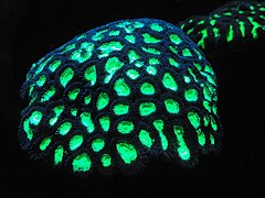  Fluorescent coral^[46]
  

Darwin's paradox

Darwin's paradox "Coral... seems to proliferate when ocean waters are warm, poor, clear and agitated, a fact which Darwin had already noted when he passed through Tahiti in 1842. This constitutes a fundamental paradox, shown quantitatively by the apparent impossibility of balancing input and output of the nutritive elements which control the coral polyp metabolism. Recent oceanographic research has brought to light the reality of this paradox by confirming that the oligotrophy of the ocean euphotic zone persists right up to the swell-battered reef crest. When you approach the reef edges and atolls from the quasidesert of the open sea, the near absence of living matter suddenly becomes a plethora of life, without transition. So why is there something rather than nothing, and more precisely, where do the necessary nutrients for the functioning of this extraordinary coral reef machine come from?"
— Francis Rougerie^[47]

In The Structure and Distribution of Coral Reefs, published in 1842, Darwin described how coral reefs were found in some areas of the tropical seas but not others, with no obvious cause. The largest and strongest corals grew in parts of the reef exposed to the most violent surf and corals were weakened or absent where loose sediment accumulated.^[48]

Tropical waters contain few nutrients^[49] yet a coral reef can flourish like an "oasis in the desert".^[50] This has given rise to the ecosystem conundrum, sometimes called "Darwin's paradox": "How can such high production flourish in such nutrient poor conditions?"^[51][52][53]

Coral reefs cover less than 0.1% of the surface of the world’s ocean, about half the land area of France, yet they support over one-quarter of all marine species. This diversity results in complex food webs, with large predator fish eating smaller forage fish that eat yet smaller zooplankton and so on. However, all food webs eventually depend on plants, which are the primary producers. Coral reefs' primary productivity is very high, typically producing 5–10 grams of carbon per square meter per day (gC·m⁻²·day⁻¹) biomass.^[54][55]

One reason for the unusual clarity of tropical waters is they are deficient in nutrients and drifting plankton. Further, the sun shines year-round in the tropics, warming the surface layer, making it less dense than subsurface layers. The warmer water is separated from deeper, cooler water by a stable thermocline, where the temperature makes a rapid change. This keeps the warm surface waters floating above the cooler deeper waters. In most parts of the ocean, there is little exchange between these layers. Organisms that die in aquatic environments generally sink to the bottom, where they decompose, which releases nutrients in the form of nitrogen (N), phosphorus (P) and potassium (K). These nutrients are necessary for plant growth, but in the tropics, they do not directly return to the surface.^{[citation needed]}

Plants form the base of the food chain, and need sunlight and nutrients to grow. In the ocean, these plants are mainly microscopic phytoplankton which drift in the water column. They need sunlight for photosynthesis, which powers carbon fixation, so they are found only relatively near the surface. But they also need nutrients. Phytoplankton rapidly use nutrients in the surface waters, and in the tropics, these nutrients are not usually replaced because of the thermocline.^{[citation needed]}

Coral polyps

Explanations

Around coral reefs, lagoons fill in with material eroded from the reef and the island. They become havens for marine life, providing protection from waves and storms.

Most importantly, reefs recycle nutrients, which happens much less in the open ocean. In coral reefs and lagoons, producers include phytoplankton, as well as seaweed and coralline algae, especially small types called turf algae, which pass nutrients to corals.^[56] The phytoplankton are eaten by fish and crustaceans, who also pass nutrients along the food web. Recycling ensures fewer nutrients are needed overall to support the community.

Coral reefs support many symbiotic relationships. In particular, zooxanthellae provide energy to coral in the form of glucose, glycerol, and amino acids.^[57] Zooxanthellae can provide up to 90% of a coral’s energy requirements.^[38] In return, as an example of mutualism, the corals shelter the zooxanthellae, averaging one million for every cubic centimeter of coral, and provide a constant supply of the carbon dioxide they need for photosynthesis.

The color of corals depends on the combination of brown shades provided by their zooxanthellae and pigmented proteins (reds, blues, greens, etc.) produced by the corals themselves.

Corals also absorb nutrients, including inorganic nitrogen and phosphorus, directly from water. Many corals extend their tentacles at night to catch zooplankton that brush them when the water is agitated. Zooplankton provide the polyp with nitrogen, and the polyp shares some of the nitrogen with the zooxanthellae, which also require this element.^[56] The varying pigments in different species of zooxanthellae give them an overall brown or golden-brown appearance, and give brown corals their colors. Other pigments such as reds, blues, greens, etc. come from colored proteins made by the coral animals. Coral which loses a large fraction of its zooxanthellae becomes white (or sometimes pastel shades in corals that are richly pigmented with their own colorful proteins) and is said to be bleached, a condition which, unless corrected, can kill the coral.

Sponges are another key: they live in crevices in the coral reefs. They are efficient filter feeders, and in the Red Sea they consume about 60% of the phytoplankton that drifts by. The sponges eventually excrete nutrients in a form the corals can use.^[58]

Most coral polyps are nocturnal feeders. Here, in the dark, polyps have extended their tentacles to feed on zooplankton.

The roughness of coral surfaces is the key to coral survival in agitated waters. Normally, a boundary layer of still water surrounds a submerged object, which acts as a barrier. Waves breaking on the extremely rough edges of corals disrupt the boundary layer, allowing the corals access to passing nutrients. Turbulent water thereby promotes reef growth and branching. Without the nutritional gains brought by rough coral surfaces, even the most effective recycling would leave corals wanting in nutrients.^[59]

Studies have shown that deep nutrient-rich water entering coral reefs through isolated events may have significant effects on temperature and nutrient systems.^[60][61] This water movement disrupts the relatively stable thermocline that usually exists between warm shallow water to deeper colder water. Leichter et al. (2006)^[62] found that temperature regimes on coral reefs in the Bahamas and Florida were highly variable with temporal scales of minutes to seasons and spatial scales across depths.

Water can be moved through coral reefs in various ways, including current rings, surface waves, internal waves and tidal changes.^{[60][63][64][65]} Movement is generally created by tides and wind. As tides interact with varying bathymetry and wind mixes with surface water, internal waves are created. An internal wave is a gravity wave that moves along density stratification within the ocean. When a water parcel encounters a different density it will oscillate and create internal waves.^[66] While internal waves generally have a lower frequency than surface waves, they often form as a single wave that breaks into multiple waves as it hits a slope and moves upward.^[67] This vertical break up of internal waves causes significant diapycnal mixing and turbulence.^[68][69] Internal waves can act as nutrient pumps, bringing plankton and cool nutrient-rich water up to the surface.^{[60][65][70][71][72][73][74][75][76][77][78]}

The irregular structure characteristic of coral reef bathymetry may enhance mixing and produce pockets of cooler water and variable nutrient content.^[79] Arrival of cool, nutrient-rich water from depths due to internal waves and tidal bores has been linked to growth rates of suspension feeders and benthic algae^[65][78][80] as well as plankton and larval organisms.^[65][81] Leichter et al.^[78] proposed that the seaweed Codium isthmocladum reacts to deep water nutrient sources due to their tissues having different concentrations of nutrients dependent upon depth. Wolanski and Hamner^[72] noted aggregations of eggs, larval organisms and plankton on reefs in response to deep water intrusions. Similarly, as internal waves and bores move vertically, surface-dwelling larval organisms are carried toward the shore.^[81] This has significant biological importance to cascading effects of food chains in coral reef ecosystems and may provide yet another key to unlocking "Darwin's Paradox".
Cyanobacteria provide soluble nitrates for the reef via nitrogen fixation.^[82]

Coral reefs also often depend on surrounding habitats, such as seagrass meadows and mangrove forests, for nutrients. Seagrass and mangroves supply dead plants and animals which are rich in nitrogen and also serve to feed fish and animals from the reef by supplying wood and vegetation. Reefs, in turn, protect mangroves and seagrass from waves and produce sediment in which the mangroves and seagrass can root.^[29]

Biodiversity

Tube sponges attracting cardinal fishes, glassfishes and wrasses

Over 4,000 species of fish inhabit coral reefs.

Organisms can cover every square inch of a coral reef.

Coral reefs form some of the world's most productive ecosystems, providing complex and varied marine habitats that support a wide range of other organisms.^[83][84]Fringing reefs just below low tide level have a mutually beneficial relationship with mangrove forests at high tide level and sea grass meadows in between: the reefs protect the mangroves and seagrass from strong currents and waves that would damage them or erode the sediments in which they are rooted, while the mangroves and sea grass protect the coral from large influxes of silt, fresh water and pollutants. This level of variety in the environment benefits many coral reef animals, which, for example, may feed in the sea grass and use the reefs for protection or breeding.^[85]

Reefs are home to a large variety of animals, including fish, seabirds, sponges, cnidarians (which includes some types of corals and jellyfish), worms, crustaceans (including shrimp, cleaner shrimp, spiny lobsters and crabs), mollusks (including cephalopods), echinoderms (including starfish, sea urchins and sea cucumbers), sea squirts, sea turtles and sea snakes. Aside from humans, mammals are rare on coral reefs, with visiting cetaceans such as dolphins being the main exception. A few of these varied species feed directly on corals, while others graze on algae on the reef.^[2][56] Reef biomass is positively related to species diversity.^[86]

The same hideouts in a reef may be regularly inhabited by different species at different times of day. Nighttime predators such as cardinalfish and squirrelfish hide during the day, while damselfish, surgeonfish, triggerfish, wrasses and parrotfish hide from eels and sharks.^[23]:49

Algae

Reefs are chronically at risk of algal encroachment. Overfishing and excess nutrient supply from onshore can enable algae to outcompete and kill the coral.^[87][88] Increased nutrient levels can be a result of sewage or chemical fertilizer runoff from nearby coastal developments. Runoff can carry nitrogen and phosphorus which promote excess algae growth. Algae can sometimes out-compete the coral for space. The algae can then smother the coral by decreasing the oxygen supply available to the reef. Decreased oxygen levels can slow down coral's calcification rates weakening the coral and leaving it more susceptible to disease and degradation.^[89] In surveys done around largely uninhabited US Pacific islands, algae inhabit a large percentage of surveyed coral locations.^[90] The algal population consists of turf algae, coralline algae, and macro algae.

Sponges

Sponges are essential for the functioning of the coral reef's ecosystem. Algae and corals in coral reefs produce organic material. This is filtered through sponges which convert this organic material into small particles which in turn are absorbed by algae and corals.^[91]

Fish

Over 4,000 species of fish inhabit coral reefs.^[2] The reasons for this diversity remain unclear. Hypotheses include the "lottery", in which the first (lucky winner) recruit to a territory is typically able to defend it against latecomers, "competition", in which adults compete for territory, and less-competitive species must be able to survive in poorer habitat, and "predation", in which population size is a function of postsettlement piscivore mortality.^[92] Healthy reefs can produce up to 35 tons of fish per square kilometer each year, but damaged reefs produce much less.^[93]

Invertebrates

Sea urchins, Dotidae and sea slugs eat seaweed. Some species of sea urchins, such as Diadema antillarum, can play a pivotal part in preventing algae from overrunning reefs.^[94] Nudibranchia and sea anemones eat sponges.

A number of invertebrates, collectively called "cryptofauna," inhabit the coral skeletal substrate itself, either boring into the skeletons (through the process of bioerosion) or living in pre-existing voids and crevices. Those animals boring into the rock include sponges, bivalve mollusks, and sipunculans. Those settling on the reef include many other species, particularly crustaceans and polychaete worms.^[32]

Seabirds

Coral reef systems provide important habitats for seabird species, some endangered. For example, Midway Atoll in Hawaii supports nearly three million seabirds, including two-thirds (1.5 million) of the global population of Laysan albatross, and one-third of the global population of black-footed albatross.^[95] Each seabird species has specific sites on the atoll where they nest. Altogether, 17 species of seabirds live on Midway. The short-tailed albatross is the rarest, with fewer than 2,200 surviving after excessive feather hunting in the late 19th century.^[96]

Other

Sea snakes feed exclusively on fish and their eggs.^[97][98][99] Marine birds, such as herons, gannets, pelicans and boobies, feed on reef fish. Some land-based reptiles intermittently associate with reefs, such as monitor lizards, the marine crocodile and semiaquatic snakes, such as Laticauda colubrina. Sea turtles, particularly hawksbill sea turtles, feed on sponges.^{[100][101][102]}

• 

  Schooling reef fish
  
• 

  Caribbean reef squid
  
• 

  Banded coral shrimp
  
• 

  Whitetip reef shark
  
• 

  Green turtle
  
• 

  Giant clam
  
• 

  Soft coral, cup coral, sponges and ascidians
  
• 

  Banded sea krait
  
• 

  The shell of Latiaxis wormaldi, a coral snail
  

Importance

Coral reefs deliver ecosystem services to tourism, fisheries and coastline protection. The global economic value of coral reefs has been estimated to be between US $29.8 billion^[6] and $375 billion per year.^[7] Coral reefs protect shorelines by absorbing wave energy, and many small islands would not exist without their reefs to protect them. According to the environmental group World Wide Fund for Nature, the economic cost over a 25-year period of destroying one kilometer of coral reef is somewhere between $137,000 and $1,200,000.^[103] About six million tons of fish are taken each year from coral reefs. Well-managed coral reefs have an annual yield of 15 tons of seafood on average per square kilometer. Southeast Asia's coral reef fisheries alone yield about $2.4 billion annually from seafood.^[103]

To improve the management of coastal coral reefs, another environmental group, the World Resources Institute (WRI) developed and published tools for calculating the value of coral reef-related tourism, shoreline protection and fisheries, partnering with five Caribbean countries. As of April 2011, published working papers covered St. Lucia, Tobago, Belize, and the Dominican Republic, with a paper for Jamaica in preparation. The WRI was also "making sure that the study results support improved coastal policies and management planning".^[104] The Belize study estimated the value of reef and mangrove services at $395–559 million annually.^[105]

Bermuda's coral reefs provide economic benefits to the Island worth on average $722 million per year, based on six key ecosystem services, according to Sarkis et al (2010).^[106]

Threats

Island with fringing reef off Yap, Micronesia^[107]

Coral reefs are dying around the world.^[107] In particular, coral mining, agricultural and urban runoff, pollution (organic and inorganic), overfishing, blast fishing, disease, and the digging of canals and access into islands and bays are localized threats to coral ecosystems. Broader threats are sea temperature rise, sea level rise and pH changes from ocean acidification, all associated with greenhouse gas emissions. A 2014 study lists factors such as population explosion along the coast lines, overfishing, the pollution of coastal areas, global warming and invasive species among the main reasons that have put reefs in danger of extinction.^[108]

A study released in April 2013 has shown that air pollution can also stunt the growth of coral reefs; researchers from Australia, Panama and the UK used coral records (between 1880 and 2000) from the western Caribbean to show the threat of factors such as coal-burning coal and volcanic eruptions.^[109] Pollutants, such as Tributyltin, a biocide released into water from in anti-fouling paint can be toxic to corals.

In 2011, researchers suggested that "extant marine invertebrates face the same synergistic effects of multiple stressors" that occurred during the end-Permian extinction, and that genera "with poorly buffered respiratory physiology and calcareous shells", such as corals, were particularly vulnerable.^{[110][111][112]}

Rock coral on seamounts across the ocean are under fire from bottom trawling. Reportedly up to 50% of the catch is rock coral, and the practice transforms coral structures to rubble. With it taking years to regrow, these coral communities are disappearing faster than they can sustain themselves.^[113]

Another cause for the death of coral reefs is bioerosion. Various fishes graze corals, dead or alive and change the morphology of coral reefs making them more susceptible to other physical and chemical threats. It has been generally observed that only the algae growing on dead corals is eaten and the live ones are not. However, this act still destroys the top layer of coral substrate and makes it harder for the reefs to sustain.^[114]

In El Niño-year 2010, preliminary reports show global coral bleaching reached its worst level since another El Niño year, 1998, when 16% of the world's reefs died as a result of increased water temperature. In Indonesia's Aceh province, surveys showed some 80% of bleached corals died. Scientists do not yet understand the long-term impacts of coral bleaching, but they do know that bleaching leaves corals vulnerable to disease, stunts their growth, and affects their reproduction, while severe bleaching kills them.^[115] In July, Malaysia closed several dive sites where virtually all the corals were damaged by bleaching.^[116][117]

To find answers for these problems, researchers study the various factors that impact reefs. The list includes the ocean's role as a carbon dioxide sink, atmospheric changes, ultraviolet light, ocean acidification, viruses, impacts of dust storms carrying agents to far-flung reefs, pollutants, algal blooms and others. Reefs are threatened well beyond coastal areas.^{[citation needed]} Coral reefs with one type of zooxanthellae are more prone to bleaching than are reefs with another, more hardy, species.^[118]

General estimates show approximately 10% of the world's coral reefs are dead.^[119][120] About 60% of the world's reefs are at risk due to destructive, human-related activities. The threat to the health of reefs is particularly high in Southeast Asia, where 95% of reefs are at risk from local threats.^[121] By the 2030s, 90% of reefs are expected to be at risk from both human activities and climate change; by 2050, all coral reefs will be in danger.^[122]

Current research is showing that ecotourism in the Great Barrier Reef is contributing to coral disease,^[123] and that chemicals in sunscreens may contribute to the impact of viruses on zooxanthellae.^[8]

Some scientists, including those associated with the National Oceanic and Atmospheric Administration, posit that US coral reefs are likely to disappear within a few decades as a result of global warming.^[124]

Protection

A diversity of corals

Marine protected areas (MPAs) have become increasingly prominent for reef management. MPAs promote responsible fishery management and habitat protection. Much like national parks and wildlife refuges, and to varying degrees, MPAs restrict potentially damaging activities. MPAs encompass both social and biological objectives, including reef restoration, aesthetics, biodiversity, and economic benefits. However, there are very few MPAs that have actually made a substantial difference. Research in Indonesia, Philippines and Papua New Guinea shows that there is no significant difference between an MPA site and an unprotected site.^[125][126] Conflicts surrounding MPAs involve lack of participation, clashing views of the government and fisheries, effectiveness of the area, and funding.^[127] In some situations, as in the Phoenix Islands Protected Area, MPAs can also provide revenue, potentially equal to the income they would have generated without controls, as Kiribati did for its Phoenix Islands.^[128]

According to the Caribbean Coral Reefs - Status Report 1970-2012 made by the IUCN. States that; stopping overfishing especially key fishes to coral reef like parrotfish, coastal zone management which reduce human pressure on reef, (for example restricting the coastal settlement, development and tourism in coastal reef) and controlling pollution specially sewage wastage, may not only reduce coral declining but also reverse it and may let to coral reef more adaptable to changes relates to climate and acidification. The report shows that healthier reef in the Caribbean are those with large population of parrotfish in countries which protect these key fishes and sea urchins, banning fish trap and Spearfishing creating "resilient reefs".^[129]

To help combat ocean acidification, some laws are in place to reduce greenhouse gases such as carbon dioxide. The Clean Water Act puts pressure on state government agencies to monitor and limit runoff of pollutants that can cause ocean acidification. Stormwater surge preventions are also in place, as well as coastal buffers between agricultural land and the coastline. This act also ensures that delicate watershed ecosystems are intact, such as wetlands. The Clean Water Act is funded by the federal government, and is monitored by various watershed groups. Many land use laws aim to reduce CO₂ emissions by limiting deforestation. Deforestation causes erosion, which releases a large amount of carbon stored in the soil, which then flows into the ocean, contributing to ocean acidification. Incentives are used to reduce miles traveled by vehicles, which reduces the carbon emissions into the atmosphere, thereby reducing the amount of dissolved CO₂ in the ocean. State and federal governments also control coastal erosion, which releases stored carbon in the soil into the ocean, increasing ocean acidification.^[130] High-end satellite technology is increasingly being employed to monitor coral reef conditions.^[131]

Biosphere reserve, marine park, national monument and world heritage status can protect reefs. For example, Belize's barrier reef, Sian Ka'an, the Galapagos islands, Great Barrier Reef, Henderson Island, Palau and Papahānaumokuākea Marine National Monument are world heritage sites.^[132]

In Australia, the Great Barrier Reef is protected by the Great Barrier Reef Marine Park Authority, and is the subject of much legislation, including a biodiversity action plan.^[133] They have compiled a Coral Reef Resilience Action Plan. This detailed action plan consists of numerous adaptive management strategies, including reducing our carbon footprint, which would ultimately reduce the amount of ocean acidification in the oceans surrounding the Great Barrier Reef. An extensive public awareness plan is also in place to provide education on the “rainforests of the sea” and how people can reduce carbon emissions, thereby reducing ocean acidification.^[134]

Inhabitants of Ahus Island, Manus Province, Papua New Guinea, have followed a generations-old practice of restricting fishing in six areas of their reef lagoon. Their cultural traditions allow line fishing, but no net or spear fishing. The result is both the biomass and individual fish sizes are significantly larger than in places where fishing is unrestricted.^[135][136]

Restoration

Coral fragments growing on nontoxic concrete

Coral aquaculture, also known as coral farming or coral gardening, is showing promise as a potentially effective tool for restoring coral reefs, which have been declining around the world.^{[137][138][139]} The process bypasses the early growth stages of corals when they are most at risk of dying. Coral seeds are grown in nurseries, then replanted on the reef.^[140] Coral is farmed by coral farmers who live locally to the reefs and farm for reef conservation or for income.

Efforts to expand the size and number of coral reefs generally involve supplying substrate to allow more corals to find a home. Substrate materials include discarded vehicle tires, scuttled ships, subway cars, and formed concrete, such as reef balls. Reefs also grow unaided on marine structures such as oil rigs.^{[citation needed]} In large restoration projects, propagated hermatypic coral on substrate can be secured with metal pins, superglue or milliput.^[141] Needle and thread can also attach A-hermatype coral to substrate.^[142]

A substrate for growing corals referred to as Biorock is produced by running low voltage electrical currents through seawater to crystallize dissolved minerals onto steel structures. The resultant white carbonate (aragonite) is the same mineral that makes up natural coral reefs. Corals rapidly colonize and grow at accelerated rates on these coated structures. The electrical currents also accelerate formation and growth of both chemical limestone rock and the skeletons of corals and other shell-bearing organisms. The vicinity of the anode and cathode provides a high-pH environment which inhibits the growth of competitive filamentous and fleshy algae. The increased growth rates fully depend on the accretion activity.^[143]

During accretion, the settled corals display an increased growth rate, size and density, but after the process is complete, growth rate and density return to levels comparable to natural growth, and are about the same size or slightly smaller.^[143]

One case study with coral reef restoration was conducted on the island of Oahu in Hawaii. The University of Hawaii has come up with a Coral Reef Assessment and Monitoring Program to help relocate and restore coral reefs in Hawaii. A boat channel on the island of Oahu to the Hawaii Institute of Marine Biology was overcrowded with coral reefs. Also, many areas of coral reef patches in the channel had been damaged from past dredging in the channel. Dredging covers the existing corals with sand, and their larvae cannot build and thrive on sand; they can only build on to existing reefs. Because of this, the University of Hawaii decided to relocate some of the coral reef to a different transplant site. They transplanted them with the help of the United States Army divers, to a relocation site relatively close to the channel. They observed very little, if any, damage occurred to any of the colonies while they were being transported, and no mortality of coral reefs has been observed on the new transplant site, but they will be continuing to monitor the new transplant site to see how potential environmental impacts (i.e. ocean acidification) will harm the overall reef mortality rate. While trying to attach the coral to the new transplant site, they found the coral placed on hard rock is growing considerably well, and coral was even growing on the wires that attached the transplant corals to the transplant site. This gives new hope to future research on coral reef transplant sites. As a result of this coral restoration project, no environmental effects were seen from the transplantation process, no recreational activities were decreased, and no scenic areas were affected by the project. This is a great example that coral transplantation and restoration can work and thrive under the right conditions, which means there may be hope for other damaged coral reefs.^[144]

Another possibility for coral restoration is gene therapy. Through infecting coral with genetically modified bacteria, it may be possible to grow corals that are more resistant to climate change and other threats.^[145]

Reefs in the past

Ancient coral reefs

Throughout Earth history, from a few thousand years after hard skeletons were developed by marine organisms, there were almost always reefs. The times of maximum development were in the Middle Cambrian (513–501 Ma), Devonian (416–359 Ma) and Carboniferous (359–299 Ma), owing to order Rugosa extinct corals, and Late Cretaceous (100–66 Ma) and all Neogene (23 Ma–present), owing to order Scleractinia corals.

Not all reefs in the past were formed by corals: those in the Early Cambrian (542–513 Ma) resulted from calcareous algae and archaeocyathids (small animals with conical shape, probably related to sponges) and in the Late Cretaceous (100–66 Ma), when there also existed reefs formed by a group of bivalves called rudists; one of the valves formed the main conical structure and the other, much smaller valve acted as a cap.

Measurements of the oxygen isotopic composition of the aragonitic skeleton of coral reefs, such as Porites, can indicate changes in the sea surface temperature and sea surface salinity conditions of the ocean during the growth of the coral. This technique is often used by climate scientists to infer the paleoclimate of a region.^[146]

The Half Life of CO2 in Earth’s Atmosphere – Part 1

Posted on September 22, 2014 by Euan Mearns
Original link:  http://euanmearns.com/the-half-life-of-co2-in-earths-atmosphere-part-1/ 

• Sequestration of CO2 from the atmosphere can be modelled using a single exponential decay constant of 2.5% per annum. There is no modelling need to introduce a multi time constant model such as the Bern Model.
• The Bern model, favoured by the IPCC, uses four different time constants and combining these produces a decay curve that is not exponential but also matches atmosphere to emissions.
• The fact that both single exponential decline and multi-time constant models of emissions can be made to fit atmospheric evolution of CO2 means that this approach does not provide proof of process. Either or neither of these models may be correct. But combined, both of these models do provide clues as to the rate of the CO2 sequestration processes.

Single time constant, 2.5% per annum, exponential decline model gives an excellent fit between emissions (LH scale, coloured bands) and actual atmosphere (RH scale, black line). This confirms Roger Andrew’s assertion from a couple of weeks ago that it was possible to model sequestration of CO2 from the atmosphere using a single decline constant. The Blue wedge at bottom is the pre-1965 emissions stack that is also declined at 2.5% per annum. The half life of ~27 years is equivalent to a residence time for CO2 of 39 years, slightly but not significantly different to Roger’s result.

A couple of weeks ago Roger Andrews had a post called The residence time of CO2 in the atmosphere is …. 33 years? that stimulated a lot of high quality debate and for me a lot of new information came to light. This is the first part of an X part series of posts aimed at summarising what we know, aiming to zero in on “the truth” about CO2 sequestration rates from the atmosphere.

In this post (Part 1) I look at a single time constant exponential decline model, compare this with Roger’s model and the Bern model favoured by the IPCC and the climate science community. The Bern model uses 4 different time constants from fast to slow and infinity and this post illustrates how this works. I am not a mathematician and prefer visual illustration of mathematical equations.

This post has been significantly delayed since I could not get my XL model to produce the same results as Roger’s. Our models now agree but may still be providing slightly different results.

In Part 2 I will discuss the Atomic bomb 14C data and the proportional reservoir growth model put forward by Phil Chapman.

Why half life is important

We hear all the time form the climate science community that even if we stop burning fossil fuels (FF) today the CO2 we have already produced will still be in the atmosphere for centuries to come. We have already lit a long slow burning fuse that will lead us to climate Armageddon. How much of this is actually true?

What we kind of know for sure is that in 1965 the mass of CO2 in the atmosphere was roughly 2400 Gt (billion tonnes) and today (2010) it is roughly 2924 Gt. That is an increase of 524 Gt. And we also know that we have added roughly 1126 Gt of CO2 to the atmosphere through burning FF and deforestation (emissions model from Roger Andrews). And so while Man’s activities may have led to a rise in CO2 the rise is only 46% of that expected from our emissions. Earth systems have already removed at least 54%. How is this reconciled with the warnings of climatic meltdown?

To understand this requires understanding of the very complex carbon cycle, but in short, some of our emissions have been dissolved in ocean water and some have been taken up by enhanced forest and plant growth. Both of these enhanced uptakes are brought about by the increased partial pressure of CO2 in the atmosphere.

Understanding exponential decline and half life

In the context of atmospheric CO2, imagine a slug of CO2 added to the atmosphere, like manmade FF emissions, and how it may decline via sequestration into the oceans and trees. If the initial slug is absorbed by 5% in the first year, and 5% of the remaining 95% the following year and so on then the decline curve would be like that shown in Figure 1. The half life is the time it takes for 50% of the initial slug to be removed. In the case of 5% per annum decline it turns out that the half life is about 13 years (t1 in Figure 1). After another 13 years (t2) another 50% of what was there after t1 is removed and so on. As a rule of thumb, after 5 half lives have past there is hardly anything left of the original slug.

Figure 1 This chart illustrates how a pulse of 13.3 billion tonnes (Gt) of CO2 injected into the atmosphere in 1965 would decay if 5% of the remaining CO2 is removed each successive year. After 13 years (t1) 50% of the pulse has been sequestered. 50% of the remainder is sequestered in the following 13 years (t2) and so on.

The residence time is defined as follows:

Half life / 0.693 = Residence time

My XL spread sheet model has the exponential decline rate as the main input variable where:

P2 = P1*r
P1 = initial amount
P2 = amount remaining after 1 year
r = the annual decline rate. For example, for annual decline of 5% r=0.95

My spread sheet gives the same result as the general decline formula:

P(t) = P0*e^-rt
P0 = initial amount
P(t) = the amount remaining after time – t
t = time in years
r = the decay rate

It also allows me to estimate half life from the output. Therefore in this discussion I will stick to using decline rate and half life as illustrated in Figure 1 and where possible avoid using the more abstract residence time term.

Single time constant, multi pulse model for the atmosphere

This may sound complicated but I hope to make it simple to understand. Roger already laid the groundwork with a chart that shows the same as Figure 2. In Figure 2, the single pulse declining at 5% per annum (Figure 1) is the layer labelled as (1) in 1965 (Figure 2). The next year there is a new pulse (2) that declines at the same rate and the next year another pulse (3) and so on. The size of each annual pulse equals emissions for that year. So we have multiple pulses but they all decline at the same rate of 5% per annum. After 13 years, half of pulse one is gone and so forth. In the 16 years shown in Figure 2 a total of 289 Gt of CO2 is added to the atmosphere but sequestration has removed 70 Gt meaning that only 210 Gt remain, that is the height of the 1980 column.

Figure 2 In his earlier post, Roger produced a chart near identical to this and one reason for reproducing this here is to show that we are both singing from the same spread sheet. The pulse shown in Figure 1 is that labeled as number (1) on the chart. The next year there is a new pulse, scaled to the emissions model, that also decays at 5% and so forth. Because of sequestration into the oceans and biosphere the amount of CO2 left in the atmosphere is always much lower than the amount we have added.

We can now expand this model to a full time series, 1965 to 2010 and adjust the exponential decline rate that the model uses to produce a best fit between the model and the observed evolution of CO2 in the atmosphere (Figure 3). The atmosphere model is based on 750 Gt C in the atmosphere in 1998 (IPCC Grid Arendal) when the atmosphere had 367 ppm CO2. The C content of the atmosphere is then projected backwards and forwards from that date in proportion to annual CO2 concentrations from Mauna Loa. The data are then converted to Gt CO2 by multiplying by 44/12 (the molecular weight of CO2 / atomic weight of carbon).

Figure 3 The model is now expanded to include all years from 1965 to 2010. The black line (right hand scale) is the atmosphere based on observed CO2 at Mauna Loa. The decline rate was adjusted to give this “best fit”. Notably 1126Gt CO2 has been added but only 516 Gt remains and this fits the overall observation of CO2 sequestration reducing emissions by 54%. In detail, the fit of the emissions to the atmosphere is not as good as that achieved by Roger.

It was at this point that I encountered the first problem trying to reconcile my model with Roger’s model. The fit of additions to atmosphere is nothing like as good as that achieved by Roger and the half life yields a residence time of  18.8 years somewhat different to Roger’s 33 years. The problem with the model shown in Figure 3 is that it is built on a flat baseline that does not account for the decline (sequestration) of pre-1965 emissions.
Building in decline to the pre-1965 emissions produces an excellent fit of emissions and the actual evolution of the atmosphere (black line) with a half life of 27 years equivalent to a residence time of 39 years. Closer to but not exactly the same as Roger’s result (Figure 4).

Figure 4 Single time constant, 2.5% per annum, exponential decline model gives an excellent fit between emissions (LH scale, coloured bands) and actual atmosphere (RH scale, black line). This confirms Roger Andrew’s assertion from a couple of weeks ago that it was possible to model sequestration of CO2 from the atmosphere using a single decline constant. The Blue wedge at bottom is the pre-1965 emissions stack that is also declined at 2.5% per annum. The half life of ~27 years is equivalent to a residence time for CO2 of 39 years.

A major conclusion of this post, therefore, is that emissions can be fitted to the observed evolution of the atmosphere using a single time constant model that has a 2.5% per annum decline rate. This credit really has to go to Roger Andrews if no one else has achieved this before. To achieve this fit, it is essential to have a model where the longer term emissions also decline. In my model, the emissions are initiated in 1910.

At this point it is important to stress that matching emissions to observations assumes that all of the rise in atmospheric CO2 comes from emissions. As we shall see in Part 2, the atomic bomb 14C data suggests a much more rapid decline of 7% per year that yields a half life of ~5 years  that creates the need for some of the increase in CO2 to come from other sources. I hope to show why the bomb data give a false picture.

This leads into consideration of the Bern Model which has multiple time constants. If it is possible to get a good model fit using a single time constant why use 4? Doing so has lead to much debate on sceptic blogs since  it is difficult to conceptualise why different processes should discriminate between different parts of the overall CO2 budget. For example Willis Eschenbach writing on WUWT:

So my question is, how do the sinks know the difference? Why don’t the fast-acting sinks just soak up the excess CO2, leaving nothing for the long-term, slow-acting sinks? I mean, if some 13% of the CO2 excess is supposed to hang around in the atmosphere for 371.3 years … how do the fast-acting sinks know to not just absorb it before the slow sinks get to it?

The Bern Model

I have not found it easy to find information on the Bern model simply through Google. And it is worth declaring that until a few weeks ago I had barely heard of it. I have this from Clive Best via email:

AR4 page 213 of WG1 defines the BERN model as
a0 + sum(i=1,3)(ai.exp(-t/Taui)) , Where a0 = 0.217, a1 = 0.259, a2 = 0.338, a3 = 0.186, Tau1 = 172.9 years, Tau2 = 18.51 years, and Tau3 = 1.186 years.
The term a0 is the fraction which remains for ever in the atmosphere ( tau = infinity) – roughly 22%

Of course it doesn’t stay in the atmosphere for ever. It is eventually removed through rock weathering and build up of  sediments on the ocean floor. Tau > 1000 years.

This is translated into the following:

Time constant (Tau)   % of annual pulse removed at that rate

1.2 y                                18%
18.5 y                             34%
173 y                              26%
∞                                    22%

The Bern model may therefore be described as a multi pulse multi time constant model. In real terms it says that certain processes will sequester CO2 emissions very quickly, for example solution into ocean water, some act more slowly, for example removal by tree growth and soils and some will act very slowly, for example removal of surface water CO2 into the deep oceans.

Figures  5, 6, 7 and 8 show what these different time slices weighted according to the % of emissions they apply to look like. Note the variable Y-axis scales, the very fast slice accounts for virtually none of the accumulated CO2 growth. These models are built on a flat baseline and so are for illustrative purposes only.

Figure 5 The super fast time constant removes most of annual CO2 additions within 5 years. This is represented by the thin yellow band in Figure 9.

Figure 6 The second time constant of 18.5 years applied to 34% of emissions is the only one that resembles the single time constant, single pulse model (Figure 3). Note this is slightly convex up while the next two charts are concave up and combining the two provides a way of producing the observed linear increase in CO2.

Figure 7 With the spread sheet model I’m using it is difficult to model the t173 year slice so I set the decline to 0.1%. With the 45 year time scale involved from 1965 to 2010 this makes little to no difference. While Figure 5 shows little carry over from one year to the next the T173 slice shows virtually 100% carry over from one year to the next. The concave up style of this slice cancels the convex up style of the T18.5 year slice.

Figure 8 The T∞ slice has decline set to 0 and is virtually the same as the T173 model shown in Figure 7.

Adding the 4 time constant slices together provides the picture shown in Figure 9.

Figure 9 Combing the slices shown in Figures 5, 6, 7 and 8 produces the picture shown here. It is important to understand that this is a picture of what remains, not what went in. Tweaking the input variables of the Bern model or the atmosphere model it should be quite straight forward to produce a better fit. The pre-1965 emissions (underlying decline) are modelled as a single exponential which is an approximation since Bern is not an exponential decline model. It would be a lot of work to adapt my spread sheet to handle the underlying decline in the proper way. Doing so would likely improve the fit. The purpose here is to illustrate how the model works.

So where does this leave our understanding? Since CO2 emissions can be matched to atmosphere evolution using different modelling approaches it is clear that the approach of matching model to observations provides no proof of the underlying process. In the Bern model, 48% of emissions remain in the atmosphere for a long time. I do not believe that the model itself provides any evidence that this is the case.

In this comment to Roger’s post Phil Chapman presented an idea of redistribution of a slug of CO2 between the fast reservoirs. The atmosphere began with 21% of the fast reservoir CO2 and Phil argued that following multiple slugs, once equilibrium was reached, the atmosphere would end up with 21% of the increased amount of CO2 circulating between the fast reservoirs (assuming linear processes). In other words, 21% of emissions will remain in the atmosphere until the slow fluxes have time to remove it. This idea rhymes with the Bern model and I am currently thinking along the lines of a model that does not decline to zero but to 21% above the original baseline.

What about Willis Eschenbach’s enigma? At the moment I think it may be helpful to think about this from a different angle. We seem to know that different processes remove CO2 at different rates. They are all acting simultaneously. Hence, maybe some of the slow processes get to CO2 emissions before the faster processes grab them? But it is possible that sequestration is dominated by fast processes, just that at equilibrium 21% of emissions may remain.

In part 2 I hope to illustrate using simple models why the bomb 14C cannot be used to model CO2 sequestration rates. And I currently believe that for the same reasons natural variations in d13C are unlikely to be useful tracers either. I will also take a closer look at Phil Chapman’s idea (I do not know if this is originally Phil’s idea) and see how this may be incorporated into a refined model.

Half-life

From Wikipedia, the free encyclopedia

Number of half-lives elapsed	Fraction remaining	Percentage remaining
0	1⁄1	100
1	1⁄2	50
2	1⁄4	25
3	1⁄8	12	.5
4	1⁄16	6	.25
5	1⁄32	3	.125
6	1⁄64	1	.563
7	1⁄128	0	.781
...	...	...
n	1/2n	100⁄(2n)

Half-life (symbol t_1⁄2) is the time required for a quantity to reduce to half its initial value. The term is commonly used in nuclear physics to describe how quickly unstable atoms undergo, or how long stable atoms survive, radioactive decay. The term is also used more generally to characterize any type of exponential or non-exponential decay. For example, the medical sciences refer to the biological half-life of drugs and other chemicals in the human body. The converse of half-life is doubling time.
The original term, half-life period, dating to Ernest Rutherford's discovery of the principle in 1907, was shortened to half-life in the early 1950s.^[1] Rutherford applied the principle of a radioactive element's half-life to studies of age determination of rocks by measuring the decay period of radium to lead-206.
Half-life is constant over the lifetime of an exponentially decaying quantity, and it is a characteristic unit for the exponential decay equation. The accompanying table shows the reduction of a quantity as a function of the number of half-lives elapsed.

Probabilistic nature

Simulation of many identical atoms undergoing radioactive decay, starting with either 4 atoms per box (left) or 400 (right). The number at the top is how many half-lives have elapsed. Note the consequence of the law of large numbers: with more atoms, the overall decay is more regular and more predictable.

A half-life usually describes the decay of discrete entities, such as radioactive atoms. In that case, it does not work to use the definition that states "half-life is the time required for exactly half of the entities to decay". For example, if there is just one radioactive atom, and its half-life is one second, there will not be "half of an atom" left after one second.

Instead, the half-life is defined in terms of probability: "Half-life is the time required for exactly half of the entities to decay on average". In other words, the probability of a radioactive atom decaying within its half-life is 50%.

For example, the image on the right is a simulation of many identical atoms undergoing radioactive decay. Note that after one half-life there are not exactly one-half of the atoms remaining, only approximately, because of the random variation in the process. Nevertheless, when there are many identical atoms decaying (right boxes), the law of large numbers suggests that it is a very good approximation to say that half of the atoms remain after one half-life.

There are various simple exercises that demonstrate probabilistic decay, for example involving flipping coins or running a statistical computer program.^[2][3][4]

Formulas for half-life in exponential decay

An exponential decay can be described by any of the following three equivalent formulas:

${\displaystyle {\begin{aligned}N(t)&=N_{0}\left({\frac {1}{2}}\right)^{\frac {t}{t_{1/2}}}\\N(t)&=N_{0}e^{-{\frac {t}{\tau }}}\\N(t)&=N_{0}e^{-\lambda t}\end{aligned}}}$

where

• N₀ is the initial quantity of the substance that will decay (this quantity may be measured in grams, moles, number of atoms, etc.),
• N(t) is the quantity that still remains and has not yet decayed after a time t,
• t_1⁄2 is the half-life of the decaying quantity,
• τ is a positive number called the mean lifetime of the decaying quantity,
• λ is a positive number called the decay constant of the decaying quantity.

The three parameters t_1⁄2, τ, and λ are all directly related in the following way:

${\displaystyle t_{1/2}={\frac {\ln(2)}{\lambda }}=\tau \ln(2)}$

where ln(2) is the natural logarithm of 2 (approximately 0.693).

By plugging in and manipulating these relationships, we get all of the following equivalent descriptions of exponential decay, in terms of the half-life:

${\displaystyle {\begin{aligned}N(t)&=N_{0}\left({\frac {1}{2}}\right)^{\frac {t}{t_{1/2}}}=N_{0}2^{-t/t_{1/2}}\\&=N_{0}e^{-t\ln(2)/t_{1/2}}\\t_{1/2}&={\frac {t}{\log _{2}(N_{0}/N(t))}}={\frac {t}{\log _{2}(N_{0})-\log _{2}(N(t))}}\\&={\frac {1}{\log _{2^{t}}(N_{0})-\log _{2^{t}}(N(t))}}={\frac {t\ln(2)}{\ln(N_{0})-\ln(N(t))}}\end{aligned}}}$

Regardless of how it's written, we can plug into the formula to get

• ${\displaystyle N(0)=N_{0}}$ as expected (this is the definition of "initial quantity")
• ${\displaystyle N\left(t_{1/2}\right)={\frac {1}{2}}N_{0}}$ as expected (this is the definition of half-life)
• ${\displaystyle \lim _{t\to \infty }N(t)=0}$; i.e., amount approaches zero as t approaches infinity as expected (the longer we wait, the less remains).

Decay by two or more processes

Some quantities decay by two exponential-decay processes simultaneously. In this case, the actual half-life T_1⁄2 can be related to the half-lives t₁ and t₂ that the quantity would have if each of the decay processes acted in isolation:

${\displaystyle {\frac {1}{T_{1/2}}}={\frac {1}{t_{1}}}+{\frac {1}{t_{2}}}}$

For three or more processes, the analogous formula is:

${\displaystyle {\frac {1}{T_{1/2}}}={\frac {1}{t_{1}}}+{\frac {1}{t_{2}}}+{\frac {1}{t_{3}}}+\cdots }$

Examples

Half life demonstrated using dice in a classroom experiment

There is a half-life describing any exponential-decay process. For example:

• The current flowing through an RC circuit or RL circuit decays with a half-life of RCln(2) or ln(2)L/R, respectively. For this example, the term half time might be used instead of "half life", but they mean the same thing.
• In a first-order chemical reaction, the half-life of the reactant is ln(2)/λ, where λ is the reaction rate constant.
• In radioactive decay, the half-life is the length of time after which there is a 50% chance that an atom will have undergone nuclear decay. It varies depending on the atom type and isotope, and is usually determined experimentally. See List of nuclides.

The half life of a species is the time it takes for the concentration of the substance to fall to half of its initial value.

In non-exponential decay

The decay of many physical quantities is not exponential—for example, the evaporation of water from a puddle, or (often) the chemical reaction of a molecule. In such cases, the half-life is defined the same way as before: as the time elapsed before half of the original quantity has decayed. However, unlike in an exponential decay, the half-life depends on the initial quantity, and the prospective half-life will change over time as the quantity decays.

As an example, the radioactive decay of carbon-14 is exponential with a half-life of 5,730 years. A quantity of carbon-14 will decay to half of its original amount (on average) after 5,730 years, regardless of how big or small the original quantity was. After another 5,730 years, one-quarter of the original will remain. On the other hand, the time it will take a puddle to half-evaporate depends on how deep the puddle is. Perhaps a puddle of a certain size will evaporate down to half its original volume in one day. But on the second day, there is no reason to expect that one-quarter of the puddle will remain; in fact, it will probably be much less than that. This is an example where the half-life reduces as time goes on. (In other non-exponential decays, it can increase instead.)

The decay of a mixture of two or more materials which each decay exponentially, but with different half-lives, is not exponential. Mathematically, the sum of two exponential functions is not a single exponential function. A common example of such a situation is the waste of nuclear power stations, which is a mix of substances with vastly different half-lives. Consider a mixture of a rapidly decaying element A, with a half-life of 1 second, and a slowly decaying element B, with a half-life of 1 year. In a couple of minutes, almost all atoms of element A will have decayed after repeated halving of the initial number of atoms, but very few of the atoms of element B will have done so as only a tiny fraction of its half-life has elapsed. Thus, the mixture taken as a whole will not decay by halves.

In biology and pharmacology

A biological half-life or elimination half-life is the time it takes for a substance (drug, radioactive nuclide, or other) to lose one-half of its pharmacologic, physiologic, or radiological activity. In a medical context, the half-life may also describe the time that it takes for the concentration of a substance in blood plasma to reach one-half of its steady-state value (the "plasma half-life"). The relationship between the biological and plasma half-lives of a substance can be complex, due to factors including accumulation in tissues, active metabolites, and receptor interactions.^[5]

While a radioactive isotope decays almost perfectly according to so-called "first order kinetics" where the rate constant is a fixed number, the elimination of a substance from a living organism usually follows more complex chemical kinetics.

For example, the biological half-life of water in a human being is about 9 to 10 days,^{[citation needed]} though this can be altered by behavior and various other conditions. The biological half-life of cesium in human beings is between one and four months.

Bandwagon effect

A literal "bandwagon", from which the metaphor is derived.

The bandwagon effect is a phenomenon whereby the rate of uptake of beliefs, ideas, fads and trends increases the more that they have already been adopted by others. In other words, the bandwagon effect is characterized by the probability of individual adoption increasing with respect to the proportion who have already done so.^[1] As more people come to believe in something, others also "hop on the bandwagon" regardless of the underlying evidence.

The tendency to follow the actions or beliefs of others can occur because individuals directly prefer to conform, or because individuals derive information from others. Both explanations have been used for evidence of conformity in psychological experiments. For example, social pressure has been used to explain Asch's conformity experiments,^[2] and information has been used to explain Sherif's autokinetic experiment.^[3]

According to this concept, the increasing popularity of a product or phenomenon encourages more people to "get on the bandwagon", too. The bandwagon effect explains why there are fashion trends.^[4]

When individuals make rational choices based on the information they receive from others, economists have proposed that information cascades can quickly form in which people decide to ignore their personal information signals and follow the behavior of others.^[5] Cascades explain why behavior is fragile—people understand that they are based on very limited information. As a result, fads form easily but are also easily dislodged. Such informational effects have been used to explain political bandwagons.^[6]

Origin

The definition of a bandwagon is a wagon which carries a band during the course of a parade, circus or other entertainment event.^[7] The phrase "jump on the bandwagon" first appeared in American politics in 1848 when Dan Rice, a famous and popular circus clown of the time, used his bandwagon and its music to gain attention for his political campaign appearances. As his campaign became more successful, other politicians strove for a seat on the bandwagon, hoping to be associated with his success. Later, during the time of William Jennings Bryan's 1900 presidential campaign, bandwagons had become standard in campaigns,^[8] and the phrase "jump on the bandwagon" was used as a derogatory term, implying that people were associating themselves with success without considering that with which they associated themselves.

In politics

The bandwagon effect occurs in voting:^[9] some people vote for those candidates or parties who are likely to succeed (or are proclaimed as such by the media), hoping to be on the "winner's side" in the end.^{[citation needed]} The bandwagon effect has been applied to situations involving majority opinion, such as political outcomes, where people alter their opinions to the majority view.^[10] Such a shift in opinion can occur because individuals draw inferences from the decisions of others, as in an informational cascade.^{[citation needed]}

Because of time zones, election results are broadcast in the eastern parts of the United States while polls are still open in the west. This difference has led to research on how the behavior of voters in western United States is influenced by news about the decisions of voters in other time zones. In 1980, NBC News declared Ronald Reagan to be the winner of the presidential race on the basis of the exit polls several hours before the voting booths closed in the west.

It is also said to be important in the American presidential primary elections. States all vote at different times, spread over some months, rather than all on one day. Some states (Iowa, New Hampshire) have special precedence to go early while others choose to wait until a certain date. This is often said to give undue influence to these states, a win in these early states is said to give a candidate the "Big Mo" (momentum) and has propelled many candidates to win the nomination. Because of this, other states often try front loading (going as early as possible) to make their say as influential as they can. In the 2008 presidential primaries two states had all or some of their delegates banned from the convention by the central party organizations for voting too early.^[11][12]

Several studies have tested this theory of the bandwagon effect in political decision making. In the 1994 study of Robert K. Goidel and Todd G. Shields in The Journal of Politics, 180 students at the University of Kentucky were randomly assigned to nine groups and were asked questions about the same set of election scenarios. About 70% of subjects received information about the expected winner.^[13] Independents, which are those who do not vote based on the endorsement of any party and are ultimately neutral, were influenced strongly in favor of the person expected to win.^[14] Expectations played a significant role throughout the study. It was found that independents are twice as likely to vote for the Republican candidate when the Republican is expected to win. From the results, it was also found that when the Democrat was expected to win, independent Republicans and weak Republicans were more likely to vote for the Democratic candidate.^[15]

A study by Albert Mehrabian, reported in the Journal of Applied Social Psychology (1998), tested the relative importance of the bandwagon (rally around the winner) effect versus the underdog (empathic support for those trailing) effect. Bogus poll results presented to voters prior to the 1996 Republican primary clearly showed the bandwagon effect to predominate on balance. Indeed, approximately 6% of the variance in the vote was explained in terms of the bogus polls, showing that poll results (whether accurate or inaccurate) can significantly influence election results in closely contested elections. In particular, assuming that one candidate "is an initial favorite by a slim margin, reports of polls showing that candidate as the leader in the race will increase his or her favorable margin".^[16] Thus, as poll results are repeatedly reported, the bandwagon effect will tend to snowball and become a powerful aid to leading candidates.

During the 1992 U.S. presidential election, Vicki G. Morwitz and Carol Pluzinski conducted a study, which was published in The Journal of Consumer Research (1996). At a large northeastern university, some of 214 volunteer business students were given the results of student and national polls indicating that Bill Clinton was in the lead. Others were not exposed to the results of the polls. Several students who had intended to vote for Bush changed their minds after seeing the poll results.^[17]

Additionally, British polls have shown an increase to public exposure. Sixty-eight percent of voters had heard of the general election campaign results of the opinion poll in 1979. In 1987, this number of voters aware of the results increased to 74%.^[18] According to British studies, there is a consistent pattern of apparent bandwagon effects for the leading party.

In microeconomics

In microeconomics, bandwagon effect describes interactions of demand and preference.^[19] The bandwagon effect arises when people's preference for a commodity increases as the number of people buying it increases. This interaction potentially disturbs the normal results of the theory of supply and demand, which assumes that consumers make buying decisions solely based on price and their own personal preference.
Gary Becker has even argued that the bandwagon effect could be so strong as to make the demand curve slope upward.^[20]

In medicine

Medical bandwagons have been identified as “the overwhelming acceptance of unproved but popular ideas”. They have led to inappropriate therapies for numerous numbers of patients, and have impeded the development of more appropriate treatment.

In Lawrence Cohen and Henry Rothschild's exposition The Bandwagons of Medicine (1979) several of these therapeutic misadventures, some of which persisted for centuries before they were abandoned, substituted by another bandwagon, or replaced by a scientifically valid alternative.^[21] The ancient serpent cult of Aesculapius, in which sacred snakes licked the afflicted as treatment of their diseases, is an example of a bandwagon gathering momentum based on a strong personality, in this case a Roman god.^[22]

In sport

Stephen Curry, two-time NBA MVP (2014/15 - 2015/16)

One who supports a particular sports team, despite having shown no interest in that team until it started gaining success, can be considered a "bandwagon fan". One recent example in the United States is the Golden State Warriors, who rose to prominence by winning the 2015 NBA Finals, followed by a record-breaking 73-9 record the following year.^[23] The bandwagon effect can be seen in the statistics of the sales of point guard Stephen Curry's jersey. Curry merchandise sales in the first two weeks of the 2015–2016 season were 453% higher than in the first two weeks of the 2014–2015 season, including a 581% increase in sales of his jersey; his merchandise was a top-seller in 38 of the 50 U.S. states, and the Warriors' merchandise became the best-selling of any NBA team.^[24]