Search This Blog

Saturday, December 15, 2018

Ganymede (moon -- updated)

From Wikipedia, the free encyclopedia

Ganymede
Ganymede g1 true-edit1.jpg
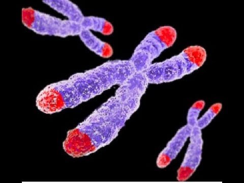
Image of Ganymede's anti-Jovian hemisphere taken by the Galileo orbiter (contrast is enhanced). Lighter surfaces, such as in recent impacts, grooved terrain and the whitish north polar cap at upper right, are enriched in water ice.
Discovery
Discovered byGalileo Galilei
Discovery dateJanuary 7, 1610
Designations
Jupiter III
AdjectivesGanymedian, Ganymedean
Orbital characteristics
Periapsis1069200 km
Apoapsis1071600 km
1070400 km
Eccentricity0.0013
7.15455296 d
Average orbital speed
10.880 km/s
Inclination2.214° (to the ecliptic)
0.20° (to Jupiter's equator)
Satellite ofJupiter
Physical characteristics
Mean radius
2634.1±0.3 km (0.413 Earths)
8.72×10⁷ km2 (0.171 Earths)
Volume7.66×1010 km3 (0.0704 Earths)
Mass1.4819×1023 kg (0.025 Earths)
Mean density
1.936 g/cm3
1.428 m/s2 (0.146 g)
0.3105±0.0028 (estimate)
2.741 km/s
synchronous
0–0.33°
Albedo0.43±0.02
Surface temp. min mean max
K 70 110 152
4.61 (opposition)
4.38 (in 1951)
Atmosphere
Surface pressure
0.2–1.2 µPa
Composition by volumeOxygen

Ganymede /ˈɡænɪmd/ (Jupiter III) is the largest and most massive moon of Jupiter and in the Solar System. The ninth largest object in the Solar System, it is the largest without a substantial atmosphere. It has a diameter of 5,268 km (3,273 mi) and is 8% larger than the planet Mercury, although only 45% as massive. Possessing a metallic core, it has the lowest moment of inertia factor of any solid body in the Solar System and is the only moon known to have a magnetic field. It is the third of the Galilean moons, the first group of objects discovered orbiting another planet, and the seventh satellite outward from Jupiter. Ganymede orbits Jupiter in roughly seven days and is in a 1:2:4 orbital resonance with the moons Europa and Io, respectively.

Ganymede is composed of approximately equal amounts of silicate rock and water ice. It is a fully differentiated body with an iron-rich, liquid core, and an internal ocean that may contain more water than all of Earth's oceans combined. Its surface is composed of two main types of terrain. Dark regions, saturated with impact craters and dated to four billion years ago, cover about a third of the satellite. Lighter regions, crosscut by extensive grooves and ridges and only slightly less ancient, cover the remainder. The cause of the light terrain's disrupted geology is not fully known, but was likely the result of tectonic activity due to tidal heating.

Ganymede's magnetic field is probably created by convection within its liquid iron core. The meager magnetic field is buried within Jupiter's much larger magnetic field and would show only as a local perturbation of the field lines. The satellite has a thin oxygen atmosphere that includes O, O2, and possibly O3 (ozone). Atomic hydrogen is a minor atmospheric constituent. Whether the satellite has an ionosphere associated with its atmosphere is unresolved.

Ganymede's discovery is credited to Galileo Galilei, who was the first to observe it on January 7, 1610. The satellite's name was soon suggested by astronomer Simon Marius, after the mythological Ganymede, cupbearer of the Greek gods, kidnapped by Zeus for the purpose. Beginning with Pioneer 10, several spacecraft have explored Ganymede. The Voyager probes, Voyager 1 and Voyager 2, refined measurements of its size, while Galileo discovered its underground ocean and magnetic field. The next planned mission to the Jovian system is the European Space Agency's Jupiter Icy Moon Explorer (JUICE), due to launch in 2022. After flybys of all three icy Galilean moons, the probe is planned to enter orbit around Ganymede.

History

Chinese astronomical records report that in 365 BC, Gan De detected what might have been a moon of Jupiter, probably Ganymede, with the naked eye. However, Gan De reported the color of the companion as reddish, which is puzzling since the moons are too faint for their color to be perceived with the naked eye. Shi Shen and Gan De together made fairly accurate observations of the five major planets.

On January 7, 1610, Galileo Galilei observed what he thought were three stars near Jupiter, including what turned out to be Ganymede, Callisto, and one body that turned out to be the combined light from Io and Europa; the next night he noticed that they had moved. On January 13, he saw all four at once for the first time, but had seen each of the moons before this date at least once. By January 15, Galileo came to the conclusion that the stars were actually bodies orbiting Jupiter. He claimed the right to name the moons; he considered "Cosmian Stars" and settled on "Medicean Stars".

Size comparison of Earth, the Moon, and Ganymede.

The French astronomer Nicolas-Claude Fabri de Peiresc suggested individual names from the Medici family for the moons, but his proposal was not taken up. Simon Marius, who had originally claimed to have found the Galilean satellites, tried to name the moons the "Saturn of Jupiter", the "Jupiter of Jupiter" (this was Ganymede), the "Venus of Jupiter", and the "Mercury of Jupiter", another nomenclature that never caught on. From a suggestion by Johannes Kepler, Marius once again tried to name the moons:
[…] Then there was Ganymede, the handsome son of King Tros, whom Jupiter, having taken the form of an eagle, transported to heaven on his back, as poets fabulously tell […] the Third, on account of its majesty of light, Ganymede […]
This name and those of the other Galilean satellites fell into disfavor for a considerable time, and were not in common use until the mid-20th century. In much of the earlier astronomical literature, Ganymede is referred to instead by its Roman numeral designation, Jupiter III (a system introduced by Galileo), in other words "the third satellite of Jupiter". Following the discovery of moons of Saturn, a naming system based on that of Kepler and Marius was used for Jupiter's moons. Ganymede is the only Galilean moon of Jupiter named after a male figure—like Io, Europa, and Callisto, he was a lover of Zeus.

Orbit and rotation

Laplace resonances of Ganymede, Europa, and Io
 
Ganymede orbits Jupiter at a distance of 1,070,400 km, third among the Galilean satellites, and completes a revolution every seven days and three hours. Like most known moons, Ganymede is tidally locked, with one side always facing toward the planet, hence its day is seven days and three hours. Its orbit is very slightly eccentric and inclined to the Jovian equator, with the eccentricity and inclination changing quasi-periodically due to solar and planetary gravitational perturbations on a timescale of centuries. The ranges of change are 0.0009–0.0022 and 0.05–0.32°, respectively. These orbital variations cause the axial tilt (the angle between rotational and orbital axes) to vary between 0 and 0.33°.

Ganymede participates in orbital resonances with Europa and Io: for every orbit of Ganymede, Europa orbits twice and Io orbits four times. Conjunctions (alignment on the same side of Jupiter) between Io and Europa occur when Io is at periapsis and Europa at apoapsis. Conjunctions between Europa and Ganymede occur when Europa is at periapsis. The longitudes of the Io–Europa and Europa–Ganymede conjunctions change with the same rate, making triple conjunctions impossible. Such a complicated resonance is called the Laplace resonance.

Jupiter's Great Red Spot and Ganymede's shadow
 
The current Laplace resonance is unable to pump the orbital eccentricity of Ganymede to a higher value. The value of about 0.0013 is probably a remnant from a previous epoch, when such pumping was possible. The Ganymedian orbital eccentricity is somewhat puzzling; if it is not pumped now it should have decayed long ago due to the tidal dissipation in the interior of Ganymede. This means that the last episode of the eccentricity excitation happened only several hundred million years ago. Because Ganymede's orbital eccentricity is relatively low—on average 0.0015—tidal heating is negligible now. However, in the past Ganymede may have passed through one or more Laplace-like resonances that were able to pump the orbital eccentricity to a value as high as 0.01–0.02. This probably caused a significant tidal heating of the interior of Ganymede; the formation of the grooved terrain may be a result of one or more heating episodes.

There are two hypotheses for the origin of the Laplace resonance among Io, Europa, and Ganymede: that it is primordial and has existed from the beginning of the Solar System; or that it developed after the formation of the Solar System. A possible sequence of events for the latter scenario is as follows: Io raised tides on Jupiter, causing Io's orbit to expand (due to conservation of momentum) until it encountered the 2:1 resonance with Europa; after that the expansion continued, but some of the angular moment was transferred to Europa as the resonance caused its orbit to expand as well; the process continued until Europa encountered the 2:1 resonance with Ganymede. Eventually the drift rates of conjunctions between all three moons were synchronized and locked in the Laplace resonance.

Physical characteristics

Depiction of Ganymede centered over 45° W. longitude; dark areas are Perrine (upper) and Nicholson (lower) regiones; prominent craters are Tros (upper right) and Cisti (lower left).

Size

Ganymede is the largest and most massive moon in the Solar System. Its diameter of 5,268 km is 0.41 times that of Earth, 0.77 times that of Mars, 1.02 times that of Saturn's Titan (the second-largest moon), 1.08 times Mercury's, 1.09 times Callisto's, 1.45 times Io's and 1.51 times the Moon's. Its mass is 10% greater than Titan's, 38% greater than Callisto's, 66% greater than Io's and 2.02 times that of the Moon.

Composition

The average density of Ganymede, 1.936 g/cm3, suggests a composition of about equal parts rocky material and mostly water-ices. The mass fraction of ices is between 46–50 %, which is slightly lower than that in Callisto. Some additional volatile ices such as ammonia may also be present. The exact composition of Ganymede's rock is not known, but is probably close to the composition of L/LL type ordinary chondrites, which are characterized by less total iron, less metallic iron and more iron oxide than H chondrites. The weight ratio of iron to silicon ranges between 1.05 and 1.27 in Ganymede, whereas the solar ratio is around 1.8.

Voyager 2 view of Ganymede's anti-Jovian hemisphere; Uruk Sulcus separates dark areas Galileo Regio (right) and Marius Regio (center left). Bright rays of recent crater Osiris (bottom) are ejected ice.

Surface features

Ganymede's surface has an albedo of about 43%. Water ice seems to be ubiquitous on its surface, with a mass fraction of 50–90 %, significantly more than in Ganymede as a whole. Near-infrared spectroscopy has revealed the presence of strong water ice absorption bands at wavelengths of 1.04, 1.25, 1.5, 2.0 and 3.0 μm. The grooved terrain is brighter and has a more icy composition than the dark terrain. The analysis of high-resolution, near-infrared and UV spectra obtained by the Galileo spacecraft and from Earth observations has revealed various non-water materials: carbon dioxide, sulfur dioxide and, possibly, cyanogen, hydrogen sulfate and various organic compounds. Galileo results have also shown magnesium sulfate (MgSO4) and, possibly, sodium sulfate (Na2SO4) on Ganymede's surface. These salts may originate from the subsurface ocean.

The Ganymedian surface albedo is very asymmetric; the leading hemisphere is brighter than the trailing one. This is similar to Europa, but the reverse for Callisto. The trailing hemisphere of Ganymede appears to be enriched in sulfur dioxide. The distribution of carbon dioxide does not demonstrate any hemispheric asymmetry, although it is not observed near the poles. Impact craters on Ganymede (except one) do not show any enrichment in carbon dioxide, which also distinguishes it from Callisto. Ganymede's carbon dioxide gas was probably depleted in the past.

A sharp boundary divides the ancient dark terrain of Nicholson Regio from the younger, finely striated bright terrain of Harpagia Sulcus.
 
Enhanced-color Galileo spacecraft image of Ganymede's trailing hemisphere. The crater Tashmetum's prominent rays are at lower right, and the large ejecta field of Hershef at upper right. Part of dark Nicholson Regio is at lower left, bounded on its upper right by Harpagia Sulcus.
 
The craters Gula and Achelous (bottom), in the grooved terrain of Ganymede, with ejecta "pedestals" and ramparts.
 
Ganymede's surface is a mix of two types of terrain: very old, highly cratered, dark regions and somewhat younger (but still ancient), lighter regions marked with an extensive array of grooves and ridges. The dark terrain, which comprises about one-third of the surface, contains clays and organic materials that could indicate the composition of the impactors from which Jovian satellites accreted.

The heating mechanism required for the formation of the grooved terrain on Ganymede is an unsolved problem in the planetary sciences. The modern view is that the grooved terrain is mainly tectonic in nature. Cryovolcanism is thought to have played only a minor role, if any. The forces that caused the strong stresses in the Ganymedian ice lithosphere necessary to initiate the tectonic activity may be connected to the tidal heating events in the past, possibly caused when the satellite passed through unstable orbital resonances. The tidal flexing of the ice may have heated the interior and strained the lithosphere, leading to the development of cracks and horst and graben faulting, which erased the old, dark terrain on 70% of the surface. The formation of the grooved terrain may also be connected with the early core formation and subsequent tidal heating of Ganymede's interior, which may have caused a slight expansion of Ganymede by 1–6 % due to phase transitions in ice and thermal expansion. During subsequent evolution deep, hot water plumes may have risen from the core to the surface, leading to the tectonic deformation of the lithosphere. Radiogenic heating within the satellite is the most relevant current heat source, contributing, for instance, to ocean depth. Research models have found that if the orbital eccentricity were an order of magnitude greater than currently (as it may have been in the past), tidal heating would be a more substantial heat source than radiogenic heating.

Cratering is seen on both types of terrain, but is especially extensive on the dark terrain: it appears to be saturated with impact craters and has evolved largely through impact events. The brighter, grooved terrain contains many fewer impact features, which have been only of a minor importance to its tectonic evolution. The density of cratering indicates an age of 4 billion years for the dark terrain, similar to the highlands of the Moon, and a somewhat younger age for the grooved terrain (but how much younger is uncertain). Ganymede may have experienced a period of heavy cratering 3.5 to 4 billion years ago similar to that of the Moon. If true, the vast majority of impacts happened in that epoch, whereas the cratering rate has been much smaller since. Craters both overlay and are crosscut by the groove systems, indicating that some of the grooves are quite ancient. Relatively young craters with rays of ejecta are also visible. Ganymedian craters are flatter than those on the Moon and Mercury. This is probably due to the relatively weak nature of Ganymede's icy crust, which can (or could) flow and thereby soften the relief. Ancient craters whose relief has disappeared leave only a "ghost" of a crater known as a palimpsest.

One significant feature on Ganymede is a dark plain named Galileo Regio, which contains a series of concentric grooves, or furrows, likely created during a period of geologic activity.

Ganymede also has polar caps, likely composed of water frost. The frost extends to 40° latitude. These polar caps were first seen by the Voyager spacecraft. Theories on the formation of the caps include the migration of water to higher latitudes and bombardment of the ice by plasma. Data from Galileo suggests the latter is correct. The presence of a magnetic field on Ganymede results in more intense charged particle bombardment of its surface in the unprotected polar regions; sputtering then leads to redistribution of water molecules, with frost migrating to locally colder areas within the polar terrain.

Geologic map of Ganymede (February 2014). The oldest, low-albedo, cratered units are reddish brown; younger, higher-albedo units are blue if grooved and blue-green if smooth (purple is a mix of grooved and smooth).

A crater named Anat provides the reference point for measuring longitude on Ganymede. By definition, Anat is at 128° longitude. The 0° longitude directly faces Jupiter, and unless stated otherwise longitude increases toward the west.

Internal structure

Ganymede appears to be fully differentiated, with an internal structure consisting of an iron-sulfideiron core, a silicate mantle and outer layers of water ice and liquid water. The precise thicknesses of the different layers in the interior of Ganymede depend on the assumed composition of silicates (fraction of olivine and pyroxene) and amount of sulfur in the core. Ganymede has the lowest moment of inertia factor, 0.31, among the solid Solar System bodies. This is a consequence of its substantial water content and fully differentiated interior

Subsurface oceans

Artist's cut-away representation of the internal structure of Ganymede. Layers drawn to scale.
 
In the 1970s, NASA scientists first suspected that Ganymede has a thick ocean between two layers of ice, one on the surface and one beneath a liquid ocean and atop the rocky mantle. In the 1990s, NASA's Galileo mission flew by Ganymede, confirming the moon's sub-surface ocean. An analysis published in 2014, taking into account the realistic thermodynamics for water and effects of salt, suggests that Ganymede might have a stack of several ocean layers separated by different phases of ice, with the lowest liquid layer adjacent to the rocky mantle. Water–rock contact may be an important factor in the origin of life. The analysis also notes that the extreme depths involved (~800 km to the rocky "seafloor") mean that temperatures at the bottom of a convective (adiabatic) ocean can be up to 40 K higher than those at the ice–water interface. In March 2015, scientists reported that measurements with the Hubble Space Telescope of how the aurorae moved over Ganymede's surface suggest it has a subsurface ocean. A large salt-water ocean affects Ganymede's magnetic field, and consequently, its aurora. The evidence suggests that Ganymede's oceans might be the largest in the entire Solar System.

There is some speculation on the potential habitability of Ganymede's ocean.

Core

The existence of a liquid, iron–nickel-rich core provides a natural explanation for the intrinsic magnetic field of Ganymede detected by Galileo spacecraft. The convection in the liquid iron, which has high electrical conductivity, is the most reasonable model of magnetic field generation. The density of the core is 5.5–6 g/cm3 and the silicate mantle is 3.4–3.6 g/cm3. The radius of this core may be up to 500 km. The temperature in the core of Ganymede is probably 1500–1700 K and pressure up to 10 GPa (99,000 atm).

Atmosphere and ionosphere

In 1972, a team of Indian, British and American astronomers working in Java (Indonesia) and Kavalur (India) claimed that they had detected a thin atmosphere during an occultation, when it and Jupiter passed in front of a star. They estimated that the surface pressure was around 0.1 Pa (1 microbar). However, in 1979, Voyager 1 observed an occultation of the star κ Centauri during its flyby of Jupiter, with differing results. The occultation measurements were conducted in the far-ultraviolet spectrum at wavelengths shorter than 200 nm, which were much more sensitive to the presence of gases than the 1972 measurements made in the visible spectrum. No atmosphere was revealed by the Voyager data. The upper limit on the surface particle number density was found to be 1.5×109 cm−3, which corresponds to a surface pressure of less than 2.5 µPa (25 picobar). The latter value is almost five orders of magnitude less than the 1972 estimate.

False-color temperature map of Ganymede
 
Despite the Voyager data, evidence for a tenuous oxygen atmosphere (exosphere) on Ganymede, very similar to the one found on Europa, was found by the Hubble Space Telescope (HST) in 1995. HST actually observed airglow of atomic oxygen in the far-ultraviolet at the wavelengths 130.4 nm and 135.6 nm. Such an airglow is excited when molecular oxygen is dissociated by electron impacts, which is evidence of a significant neutral atmosphere composed predominantly of O2 molecules. The surface number density probably lies in the (1.2–7)×108 cm−3 range, corresponding to the surface pressure of 0.2–1.2 µPa. These values are in agreement with the Voyager's upper limit set in 1981. The oxygen is not evidence of life; it is thought to be produced when water ice on Ganymede's surface is split into hydrogen and oxygen by radiation, with the hydrogen then being more rapidly lost due to its low atomic mass. The airglow observed over Ganymede is not spatially homogeneous like that over Europa. HST observed two bright spots located in the northern and southern hemispheres, near ± 50° latitude, which is exactly the boundary between the open and closed field lines of the Ganymedian magnetosphere (see below). The bright spots are probably polar auroras, caused by plasma precipitation along the open field lines.

The existence of a neutral atmosphere implies that an ionosphere should exist, because oxygen molecules are ionized by the impacts of the energetic electrons coming from the magnetosphere and by solar EUV radiation. However, the nature of the Ganymedian ionosphere is as controversial as the nature of the atmosphere. Some Galileo measurements found an elevated electron density near Ganymede, suggesting an ionosphere, whereas others failed to detect anything. The electron density near the surface is estimated by different sources to lie in the range 400–2,500 cm−3. As of 2008, the parameters of the ionosphere of Ganymede are not well constrained. 

Additional evidence of the oxygen atmosphere comes from spectral detection of gases trapped in the ice at the surface of Ganymede. The detection of ozone (O3) bands was announced in 1996. In 1997 spectroscopic analysis revealed the dimer (or diatomic) absorption features of molecular oxygen. Such an absorption can arise only if the oxygen is in a dense phase. The best candidate is molecular oxygen trapped in ice. The depth of the dimer absorption bands depends on latitude and longitude, rather than on surface albedo—they tend to decrease with increasing latitude on Ganymede, whereas O3 shows an opposite trend. Laboratory work has found that O2 would not cluster or bubble but dissolve in ice at Ganymede's relatively warm surface temperature of 100 K (−173.15 °C).

A search for sodium in the atmosphere, just after such a finding on Europa, turned up nothing in 1997. Sodium is at least 13 times less abundant around Ganymede than around Europa, possibly because of a relative deficiency at the surface or because the magnetosphere fends off energetic particles. Another minor constituent of the Ganymedian atmosphere is atomic hydrogen. Hydrogen atoms were observed as far as 3,000 km from Ganymede's surface. Their density on the surface is about 1.5×104 cm−3.

Magnetosphere

Magnetic field of the Jovian satellite Ganymede, which is embedded into the magnetosphere of Jupiter. Closed field lines are marked with green color.
 
The Galileo craft made six close flybys of Ganymede from 1995–2000 (G1, G2, G7, G8, G28 and G29) and discovered that Ganymede has a permanent (intrinsic) magnetic moment independent of the Jovian magnetic field. The value of the moment is about 1.3 × 1013 T·m3, which is three times larger than the magnetic moment of Mercury. The magnetic dipole is tilted with respect to the rotational axis of Ganymede by 176°, which means that it is directed against the Jovian magnetic moment. Its north pole lies below the orbital plane. The dipole magnetic field created by this permanent moment has a strength of 719 ± 2 nT at Ganymede's equator, which should be compared with the Jovian magnetic field at the distance of Ganymede—about 120 nT. The equatorial field of Ganymede is directed against the Jovian field, meaning reconnection is possible. The intrinsic field strength at the poles is two times that at the equator—1440 nT.

Aurorae on Ganymede—auroral belt shifting may indicate a subsurface saline ocean.

The permanent magnetic moment carves a part of space around Ganymede, creating a tiny magnetosphere embedded inside that of Jupiter; it is the only moon in the Solar System known to possess the feature. Its diameter is 4–5 RG (RG = 2,631.2 km). The Ganymedian magnetosphere has a region of closed field lines located below 30° latitude, where charged particles (electrons and ions) are trapped, creating a kind of radiation belt. The main ion species in the magnetosphere is single ionized oxygen—O+—which fits well with Ganymede's tenuous oxygen atmosphere. In the polar cap regions, at latitudes higher than 30°, magnetic field lines are open, connecting Ganymede with Jupiter's ionosphere. In these areas, the energetic (tens and hundreds of kiloelectronvolt) electrons and ions have been detected, which may cause the auroras observed around the Ganymedian poles. In addition, heavy ions precipitate continuously on Ganymede's polar surface, sputtering and darkening the ice.

The interaction between the Ganymedian magnetosphere and Jovian plasma is in many respects similar to that of the solar wind and Earth's magnetosphere. The plasma co-rotating with Jupiter impinges on the trailing side of the Ganymedian magnetosphere much like the solar wind impinges on the Earth's magnetosphere. The main difference is the speed of plasma flow—supersonic in the case of Earth and subsonic in the case of Ganymede. Because of the subsonic flow, there is no bow shock off the trailing hemisphere of Ganymede.

In addition to the intrinsic magnetic moment, Ganymede has an induced dipole magnetic field. Its existence is connected with the variation of the Jovian magnetic field near Ganymede. The induced moment is directed radially to or from Jupiter following the direction of the varying part of the planetary magnetic field. The induced magnetic moment is an order of magnitude weaker than the intrinsic one. The field strength of the induced field at the magnetic equator is about 60 nT—half of that of the ambient Jovian field. The induced magnetic field of Ganymede is similar to those of Callisto and Europa, indicating that Ganymede also has a subsurface water ocean with a high electrical conductivity.

Given that Ganymede is completely differentiated and has a metallic core, its intrinsic magnetic field is probably generated in a similar fashion to the Earth's: as a result of conducting material moving in the interior. The magnetic field detected around Ganymede is likely to be caused by compositional convection in the core, if the magnetic field is the product of dynamo action, or magnetoconvection.

Despite the presence of an iron core, Ganymede's magnetosphere remains enigmatic, particularly given that similar bodies lack the feature. Some research has suggested that, given its relatively small size, the core ought to have sufficiently cooled to the point where fluid motions, hence a magnetic field would not be sustained. One explanation is that the same orbital resonances proposed to have disrupted the surface also allowed the magnetic field to persist: with Ganymede's eccentricity pumped and tidal heating of the mantle increased during such resonances, reducing heat flow from the core, leaving it fluid and convective. Another explanation is a remnant magnetization of silicate rocks in the mantle, which is possible if the satellite had a more significant dynamo-generated field in the past.

Origin and evolution

Ganymede probably formed by an accretion in Jupiter's subnebula, a disk of gas and dust surrounding Jupiter after its formation. The accretion of Ganymede probably took about 10,000 years, much shorter than the 100,000 years estimated for Callisto. The Jovian subnebula may have been relatively "gas-starved" when the Galilean satellites formed; this would have allowed for the lengthy accretion times required for Callisto. In contrast Ganymede formed closer to Jupiter, where the subnebula was denser, which explains its shorter formation timescale. This relatively fast formation prevented the escape of accretional heat, which may have led to ice melt and differentiation: the separation of the rocks and ice. The rocks settled to the center, forming the core. In this respect, Ganymede is different from Callisto, which apparently failed to melt and differentiate early due to loss of the accretional heat during its slower formation. This hypothesis explains why the two Jovian moons look so dissimilar, despite their similar mass and composition. Alternative theories explain Ganymede's greater internal heating on the basis of tidal flexing or more intense pummeling by impactors during the Late Heavy Bombardment. In the latter case, modeling suggests that differentiation would become a runaway process at Ganymede but not Callisto.

After formation, Ganymede's core largely retained the heat accumulated during accretion and differentiation, only slowly releasing it to the ice mantle. The mantle, in turn, transported it to the surface by convection. The decay of radioactive elements within rocks further heated the core, causing increased differentiation: an inner, ironiron-sulfide core and a silicate mantle formed. With this, Ganymede became a fully differentiated body. By comparison, the radioactive heating of undifferentiated Callisto caused convection in its icy interior, which effectively cooled it and prevented large-scale melting of ice and rapid differentiation. The convective motions in Callisto have caused only a partial separation of rock and ice. Today, Ganymede continues to cool slowly. The heat being released from its core and silicate mantle enables the subsurface ocean to exist, whereas the slow cooling of the liquid Fe–FeS core causes convection and supports magnetic field generation. The current heat flux out of Ganymede is probably higher than that out of Callisto.

Exploration

Completed missions

Ganymede from Pioneer 10 (1973)

Several probes flying by or orbiting Jupiter have explored Ganymede more closely, including four flybys in the 1970s, and multiple passes in the 1990s to 2000s.

Pioneer 10 approached in 1973 and Pioneer 11 in 1974, and they returned information about the satellite. This included more specific determination on physical characteristics and resolving features to 400 km (250 mi) on its surface. Pioneer 10's closest approach was 446,250 km.

Voyager 1 and Voyager 2 were next, passing by Ganymede in 1979. They refined its size, revealing it was larger than Saturn's moon Titan, which was previously thought to have been bigger. The grooved terrain was also seen.

In 1995, the Galileo spacecraft entered orbit around Jupiter and between 1996 and 2000 made six close flybys to explore Ganymede. These flybys are denoted G1, G2, G7, G8, G28 and G29. During the closest flyby—G2—Galileo passed just 264 km from the surface of Ganymede. During a G1 flyby in 1996, the Ganymedian magnetic field was discovered, while the discovery of the ocean was announced in 2001. Galileo transmitted a large number of spectral images and discovered several non-ice compounds on the surface of Ganymede. The most recent close observations of Ganymede were made by New Horizons, which recorded topographic and compositional mapping data of Europa and Ganymede during its flyby of Jupiter in 2007 en route to Pluto.

Mission concepts

The Europa Jupiter System Mission (EJSM) had a proposed launch date in 2020, and was a joint NASA and ESA proposal for exploration of many of Jupiter's moons including Ganymede. In February 2009 it was announced that ESA and NASA had given this mission priority ahead of the Titan Saturn System Mission. EJSM consisted of the NASA-led Jupiter Europa Orbiter, the ESA-led Jupiter Ganymede Orbiter, and possibly a JAXA-led Jupiter Magnetospheric Orbiter. ESA's contribution faced funding competition from other ESA projects, but on 2 May 2012 the European part of the mission, renamed Jupiter Icy Moon Explorer (JUICE), obtained a L1 launch slot in 2022 with an Ariane 5 in the ESA's Cosmic Vision science program. The spacecraft will orbit Ganymede and conduct multiple flyby investigations of Callisto and Europa.


The Russian Space Research Institute is currently evaluating the Ganymede Lander (GL) mission, with emphasis on astrobiology. The Ganymede Lander would be a partner mission for JUpiter ICy moon Explorer (JUICE). If selected, it would be launched in 2024, though this schedule might be revised and aligned with JUICE.

A Ganymede orbiter based on the Juno probe was proposed in 2010 for the Planetary Science Decadal Survey. Possible instruments include Medium Resolution Camera, Flux Gate Magnetometer, Visible/NIR Imaging Spectrometer, Laser Altimeter, Low and High Energy Plasma Packages, Ion and Neutral Mass Spectrometer, UV Imaging Spectrometer, Radio and Plasma Wave sensor, Narrow Angle Camera, and a Sub-Surface Radar.

Another canceled proposal to orbit Ganymede was the Jupiter Icy Moons Orbiter. It was designed to use nuclear fission for power, ion engine propulsion, and would have studied Ganymede in greater detail than previously. However, the mission was canceled in 2005 because of budget cuts. Another old proposal was called The Grandeur of Ganymede.

Computing the Origin of Life

The early Earth was a hellish place with impact galore and a choking atmosphere, and yet somehow life got a grip there. Image credit: Simone Marchi/SwRI.

As a principal investigator in the NASA Ames Exobiology Branch, Andrew Pohorille is searching for the origin of life on Earth, yet you won’t find him out in the field collecting samples or in a laboratory conducting experiments in test tubes. Instead, Pohorille studies the fundamental processes of life facing a computer.

Pohorille’s work is at the vanguard of a sea-change in how science can tackle the complex question of where life came from, how its biochemistry operates and what life elsewhere might be like. Rather than relying on the hit-and-miss of laboratory experiments, Pohorille believes that theoretical work is just as important, if not more so, in understanding how life could have emerged from non-life.

“The role of theory is twofold,” he says. “It provides explanations and generalizations of what is observed in experiments, but it also has some predictive power.”

Pohorille’s theoretical work resides within a field known as computational biology; Pohorille himself is director of the Center for Computational Astrobiology and Fundamental Biology at NASA’s Ames Research Center in Mountain View, California, and a Principal Investigator with the Exobiology & Evolutionary Biology Program. Computational biology involves designing and writing algorithms within mathematical models that seek to explain life’s complex biochemical processes. This is in comparison to ‘artificial life,’ which creates virtual life-forms that reside in the computer and which can mimic life’s processes. However, the approach of computational biology hasn’t been an instant hit with all biochemists and evolutionary biologists.

“It’s still contentious, partly because there is a group of people who do believe that [searching for] the origins of life is a strictly experimental issue that can only be solved in the lab,” says Pohorille. “I respectfully disagree with those who think that way.”

This is a view shared by Eric Smith, a researcher in complex non-equilibrium systems at the Earth-Life Science Institute (ELSI) which is attached to the Tokyo Institute of Technology in Japan. Smith highlights how, in recent years, the fields of computational biology and chemistry have matured to the point that researchers used to working in the laboratory can no longer ignore it. “I think we’re on the threshold of where it’s going to start becoming a serious tool, but it’s important to remember that it’s only one tool of many.”

An example of the usefulness of computational biology can be seen in Smith’s work delving into the origins of carbon-fixing, which describes how organisms convert inorganic carbon into the organic compounds vital to life. Smith and his colleague Rogier Braakman of the Chisholm Lab at the Massachusetts Institute of Technology combined a computational approach to phylogenetics (which is the study of the evolutionary relationships between organisms) with metabolic flux balance analysis (which allows metabolisms to be recreated in mathematical simulations on the computer) to disentangle the six different ways in which life is known to fix carbon, in the process figuring out which of the sextet evolved first. Consequently, Smith and Braakman were able to show how this form of carbon-fixing, which was one of life’s original metabolic processes, was able to arise from simple geochemistry. As such, it mirrors the overall quest for the origin of life in terms of how biological processes developed from geochemistry.

Although some of these research questions are attainable using computer modeling, we are still lacking an understanding of many of the basic rules governing biochemistry as well as early life’s genetics. Some researchers have speculated about an ‘RNA world’ wherein the self-replicating RNA molecule not only played the role that DNA, which is fashioned from RNA, does today, but that it also arose pre-biotically and was a cornerstone in the origin of life. However, many scientists, including Pohorille and Smith, disagree, claiming that RNA is too big and unwieldy a molecule to have played a role in life’s probably simpler origins. Instead, they suspect that there was some other chemistry at work in the origins of self-reproducing life, although what this chemistry could have been remains a subject of vigorous discussion.

Given this uncertainty, Pohorille favors forming generalizations about the biological processes at work in the origin and earliest evolution of life, rather than looking for specific outcomes. Using computational theory, he advocates focusing on the underlying principles of biological processes that are rooted in the laws of physics and chemistry. “What is needed are some general rules that guide us in building scenarios,” he says. “Just having individual experiments that say something is possible – because that’s as much as we can get from the experiment – is not enough.”

Artificial life

One of the biggest questions about the origin of life and its subsequent evolution is how random molecules managed to organize themselves into complex living organisms. What prompted them to form complex molecular chains that became the basis of life, and what are the underlying principles that govern which molecules became the important cogs in the system? With so many permutations of how molecules can combine, on the face it would seem extremely unlikely that nature would just stumble onto the right combination of molecules to form self-replicating life.

Chris Adami of Michigan State University is using artificial life inside a computer to attempt to understand the general principles behind the origin of self-replicating life. Image credit: Michigan State University.

At Michigan State University, Chris Adami thinks he has the answer. A professor of microbiology and molecular genetics, Adami takes computational biology to the next level by using the artificial life software called Avida, which runs self-replicating programs that mimic biology and evolution. Through Avida, which he co-developed in 1993 with his Michigan State colleague Charles Ofria and UC Davis’ Titus Brown, Adami is able to test his controversial but potentially revolutionary idea that life can be defined as ‘information that self-replicates’ and that the selection of useful molecular systems for life is governed by the laws of probability.

Avida operates by creating a virtual world in which programs compete for CPU time and memory access, just like organisms competing for resources in the real world. These virtual lifeforms can self-replicate, but crucially they have copy error programmed into them so that, just like in real life, mutations can be carried over to daughter programs to simulate evolution by natural selection. Because they are self-replicating, mutating computer programs could potentially be very dangerous were they to escape Avida and infect the Internet. As a safety precaution, the virtual world is run on a simulated computer inside a real computer so that the programs appear on the outside merely as data.

Where does the first replicator come from? In Avida the first replicator is purposefully written, but in real life the first biological replicator had to emerge spontaneously from nature, and this is where selectivity comes in. “It turns out that replicators, whether in nature or within Avida, are rare,” says Adami, “and the odds are that a random program – or assembly of molecules – will not replicate.”

The programs are written in a computer language that contains 26 instructions, analogous to individual monomers in chemistry, labelled as the letters of the alphabet from a to z. Adami uses this system to draw an analogy to the written word. Imagine a bag filled with equal numbers of all the letters of the alphabet. A random drawing of the letters into sequences of varying lengths, called ‘linear heteropolymers,’ creates strings of instructions into which information is encoded. If these polymers were meant to be ‘words,’ they would mostly be gibberish, containing a jumble of ‘q’s and ‘z’s and other letters without connoting meaning. Similarly, the molecules that were available on early Earth had many different ways to bind together to produce a variety of chemical reactions; the chance of nature generating the right molecular structure to enable self-replication is slim.

The Biased Typewriter

Adami points out though that language is loaded to favor certain letters that crop up more often than others. Seldom are ‘q’s or ‘z’s used, but ‘t’s and ‘e’s and ‘a’s are common letters in words. Adami suggests that the selection problem can be better understood as the ‘biased typewriter’ model, in which some molecules and chemical reactions are more likely to occur than others. If the letters in the bag were scrabble tiles, with more of the common letters and fewer of the rarely used letters, then even pulling them out at random would lead to some real words being produced, just by chance.

With his student Thomas LaBar, Adami tested the principle of the biased typewriter in Avida, loading the instructions with those monomers that are useful for self-replication. In a billion random programs made from chains of ‘letters’ that Avida subsequently produced, Adami found that 27 of them could self-replicate. He used those 27 to create a probability distribution and then kept running the program, finding that the number of self-replicators kept increasing dramatically.

“In other words, what this tells you is that if you have a process that generates these monomers at the right frequency, then you’re going to be able to find the self-replicators much faster,” says Adami.

Just 27 initial self-replicators out of a billion linear heteropolymers doesn’t sound like very much, but early Earth was a big place full of opportunity, with all kinds of different environments in which nature could experiment by combining monomers to form useful polymers for life. However, although Adami’s theoretical estimates have been born out experimentally by Avida, replicating the process to test the RNA World theory is a different proposition because the amount of information contained within RNA is too great even for the computer to handle. Nevertheless, Adami sees his ‘biased typewriter’ model as one of the general rules to which Pohorille was referring.

Eric Smith agrees with Adami that the basic idea behind the biased typewriter is on point.

“By biasing the building block inventory, you can drastically change the likelihood of one assembly versus another and we see it in all sorts of places in biology,” he says.

When it comes to the importance of information and the relevance of artificial life, Smith has his doubts. “One shouldn’t look for a big answer from any one piece of work,” he says. Instead, he says, the origin of life isn’t just one problem that requires an overarching solution, but an enormous sequence of problems, including the origin of all the metabolic processes as well as self-replication that must each be solved and no one model or computer program can provide the answer. Yet it was once thought that artificial life might have been able to do just that.

“People on both sides — artificial life and origins of life — don’t really pursue that much anymore,” he says. “There’s not much cross-talk between the two.”

Andrew Pohorille is also skeptical about Adami’s approach, as well as the usefulness of artificial life to origin of life research, suggesting that without some high-level mathematical concept that explains why there is only one set of rules that governs the origin of life and life’s processes, whether real or virtual, then the rules of virtual worlds like Avida will not necessarily translate into the real world.

“There may be many rules that lead to these kinds of processes,” says Pohorille. “The question is whether any of these rules have anything to do with the rules that operated at the origins of life.”

Adami acknowledges that the rules in Avida won’t be the same as the geochemical and biochemical rules that operate in real life, but he argues that regardless of the chemistry, the principles of information theory remain.

“It’s of course true that we will not find how life evolved on Earth by looking inside a computer,” he admits, “But we can test general principles and, once we know these principles, we can go ahead and test those in biochemical systems.”

How did the first self-replicating polymers, the precursors of life, come to form on the early Earth around four billion years ago? Image credit: NASA Goddard Space Flight Center Conceptual Image Lab.

Computational Astrobiology

In the laboratory researchers work with terrestrial life and observe its processes, but on alien worlds life could be very different, operating under different rules that are impossible to test with Earthly life in an experiment. Computational biology and artificial life, however, offer the unique abilities to explore life abstractly by investigating different processes that could exist on other planets with different environments and geochemistry. Could computational biology help astrobiologists describe alien life before we even find it?

NASA scientists certainly think that’s feasible, having recently invited Chris Adami to a workshop to discuss biomarkers, where he presented his idea of how to look for life through information and its replication, rather than RNA and proteins. Adami describes this research effort in terms of patterns that are unnatural or in disequilibrium, looking for letters and finding ‘e’ more common than ‘h’, as in the Avidian life example. In order to do this the local geochemistry needs to be known fairly well, which is something far beyond out current abilities of exoplanet studies.

Closer to home our knowledge of geochemistry is a little better, or at least can be improved in the near future. Take Europa, for instance. “We’re thinking about what evidence for life we should search for there,” says Pohorille. The idea is to computationally explore the range of molecules other than proteins or nucleic acids that could perform the same functions as they do on Earth, and figure out what their biosignatures would be on Europa. On a cautionary note, it might be tempting to describe something too extreme using these alternative concepts for life. “It’s kind of a dilemma,” says Pohorille. “What is enough and what is too much?”

Something might look like life in Avida, but there’s a danger of falling into the trap of looking for a pattern that resembles life, but isn’t, like confusing the motions of a slinky toy with those of a snake. It’s this concern that virtual life in the computer, such as Avidian life, may only be masquerading as representing life that causes so many researchers to be suspicious of its results. “In principle artificial life could help provide alternatives to Earth life, but you’ve got to figure out what your computer model is an abstraction of, and that’s the hard part,” says Smith.

Nevertheless, the scientific community as a whole is slowly coming around to the notion that computational biology and chemistry, as well as possibly artificial life, could be vital in progressing the field further. Smith, for example, wonders whether our understanding of the chemistry of complex systems needs to take on a cyborg-like quality by integrating a lot more closely with computational research.

Meanwhile, the field needs a new generation of scientists trained in the use and application of computers for theoretical work, something that is forthcoming now that the computational tools are available and scientists are figuring out new and innovative ways to use them.

“When I started doing these computational simulations, almost nobody could see how it could possibly be related to anything remotely interesting to the origins of life community,” admits Pohorille, saying he was tolerated by his peers because he was just “one odd guy.” Today, however, he says that younger researchers are realizing that theory and experiments have to go hand-in-hand.

If the field of computational biology is truly going to grow, the funding has to also. Currently, NASA is the only agency in the United States funding origin of life research, with some private money coming from the likes of the Simons Foundation and the Templeton Foundation. “Tell me of a university that is looking for theorists specializing in the origin of life,” asks Pohorille rhetorically. “I haven’t heard of one.” Internationally, ELSI in Japan is one of the few institutions hoping to get closer to the origin of life through computational efforts.

As computing power increases, scientists using it will increasingly be able to solve problems about life’s processes. Perhaps computational biology will be just one tool among many available to researchers, but its presence will not only help scientists to think of new ways to explore the origins of life, but also to come up with new ways to think about it too. The mystery of life’s origins could one day be solved thanks to that modern antithesis of life – the computer.

Did a new form of plague destroy Europe’s Stone Age societies?

The bacteria Yersinia pestis, which causes plague, has been killing people for at least 5000 years. SCIENCE ARTWORK/Science Source


Nearly 5000 years ago, a 20-year-old woman was buried in a tomb in Sweden, one of Europe’s early farmers dead in her prime. Now, researchers have discovered what killed her—Yersinia pestis, the bacterium that causes plague. The sample is one of the oldest ever found, and it belongs to a previously unknown branch of the Y. pestis evolutionary tree. This newly discovered strain of plague could have caused the collapse of large Stone Age settlements across Europe in what might be the world’s first pandemic, researchers on the project say. But other scientists contend there isn’t yet enough evidence to prove the case.

“Plague is starting to seem like it’s everywhere,” says Kyle Harper, a historian at the University of Oklahoma in Norman who studies how the disease affected human societies. Ancient plague genomes, such as the one in the new study, show “we have a really long history with this germ,” he says.

Until now, the oldest known strain of plague came to Europe with the Yamnaya, herders from the central Eurasian steppe who swept into the continent some 4800 years ago. That was followed, several thousand years later, by the strain that led to both the Justinian Plague, which afflicted the Roman Empire in the sixth century C.E., and the Black Death, which killed half of Europe’s population in the 1300s.

The discovery of the new strain was fortuitous. A team led by Simon Rasmussen, a computational biologist at the University of Copenhagen, and Nicolás Rascovan, a biologist at Aix-Marseille University in France, were scanning publicly available ancient DNA datasets for the genetic sequences of common human pathogens. They found Y. pestis sequences in the teeth of the 20-year-old woman, who was buried in the Frälsegården grave in western Sweden, and in the teeth of another person buried in the same grave, they report today in Cell. Both were farmers from Scandinavia’s Funnel Beaker culture, and neither had any trace of Yamnaya ancestry—meaning a form of plague was present in Europe before the steppe migrants arrived. That the bacterium was preserved in their teeth means it was circulating in their blood and very likely killed them, Rasmussen says.

A young woman who died of an early form of plague was buried in this Neolithic grave in Sweden. Karl-Göran Sjögren/University of Gothenburg

The newly discovered Neolithic bacterium belongs to a branch of the plague family tree separate from the later, better-known strains. It split off from a common ancestor about 5700 years ago, Rasmussen and Rascovan say. But it’s not the common ancestor itself, meaning it doesn’t reveal where or when plague originated, says Johannes Krause, a geneticist at the Max Planck Institute for the Science of Human History in Jena, Germany, who has also studied ancient plague. “I’m not sure we have a good sense of how far back [plague] goes,” agrees Anne Stone, an anthropological geneticist who studies ancient pathogens at Arizona State University in Tempe.

Rasmussen and Rascovan have an idea. During the Neolithic, the region in Eastern Europe that today includes Moldova, Romania, and parts of Ukraine was home to large “megasettlements” of tens of thousands of people belonging to what archaeologists call the Trypillia culture. Though their settlements weren’t complex enough to qualify as cities, their residents still lived in close quarters with poor sanitation and stores of grain that would have attracted rodents, Y. pestis’s wild host. “These megasettlements are the textbook example of a place where a pathogen could evolve,” Rasmussen says.

But about 5400 years ago, many of the megasettlements collapsed. Residents died or moved away, and the buildings they abandoned were burned. Rasmussen and Rascovan propose their new strain of plague might be the culprit. “Maybe this is the first time that a huge society collapses based on plague,” Rasmussen says. And because these megasettlements were connected to other communities all over Europe by trade routes, the bacterium could have easily spread to places such as Sweden. “This could in principle be the first pandemic,” Rasmussen says.

Still, the only way to know for sure would be to find evidence of Y. pestis in the collapsing megasettlements themselves. Without that, it’s “highly speculative,” Krause says. And this early strain does not have the genetic adaptations that made later ones so easy to catch, such as their ability to spread from rodents to humans through fleas. “Does this particular branch of Y. pestis have what it takes to cause a pandemic?” Stone wonders. Without knowing more about this strain, exactly how the 20-year-old woman caught the disease—and whether she was a victim of a wider pandemic—may remain a mystery.

*Correction, 6 December, 2:27 p.m.: This article originally stated that the ancient plague strain likely didn't affect the lungs. In fact, it could have caused pneumonic plague.

Posted in:
doi:10.1126/science.aaw2982

Scientists are one step closer to reversing the aging process entirely

This particular type of gene therapy gave mice younger bodies and 30% longer lifespans.


I'm determined to age gracefully. Though my wife plucks every gray hair she finds, I'd be bald if I did. Even so, I've kept myself up over the years, prompting my college girlfriend, whom I recently reconnected with to exclaim, “You haven't aged at all!" Except for more gray hair, that is. Perhaps it's just good genes. I've always chalked it up to stress-free living. So what can be done to overcome the aging process? Creams, lotions, and other products fill pharmacy shelves, but few have a truly substantial impact.

Now, researchers at the Salk Institute in La Jolla, California have discovered a way to turn back the hands of time. Juan Carlos Izpisua Belmonte led this study, published in the journal Cell. Here, elderly mice underwent a new sort of gene therapy for six weeks. Afterward, their injuries healed, their heart health improved, and even their spines were straighter. The mice also lived longer, 30% longer.

Today, we target individual age-related diseases when they spring up. But this study could help us develop a therapy to attack aging itself, and perhaps even target it before it begins taking shape. But such a therapy is at least ten years away, according to Izpisua Belmonte.

Many biologists now believe that the body, specifically the telomeres—the structures at the end of chromosomes, after a certain time simply wear out. Once degradation overtakes us, it's the beginning of the end. This study strengthens another theory. Over the course of a cell's life, epigenetic changes occur. This is the activation or depression of certain genes in order to allow the organism to respond better to its environment. Methylation tags are added to activate genes. These changes build up over time, slowing us down, and making us vulnerable to disease.

Chromosomes with telomeres in red.

Though we may add life to years, don't consider immortality an option, at least not in the near-term. “There are probably still limits that we will face in terms of complete reversal of aging," Izpisua Belmonte said. “Our focus is not only extension of lifespan but most importantly health-span." That means adding more healthy years to life, a noble prospect indeed.

The technique employs induced pluripotent stem cells (iPS). These are similar to those which are present in developing embryos. They are important as they can turn into any type of cell in the body. The technique was first used to turn back time on human skin cells, successfully.

By switching around four essential genes, all active inside the womb, scientists were able to turn skin cells into iPS cells. These four genes are known as Yamanaka factors. Scientists have been aware of their potential in anti-aging medicine for some time. In the next leg, researchers used genetically engineered mice who could have their Yamanaka factors manipulated easily, once they were exposed to a certain agent, present in their drinking water.

Since Yamanaka factors reset genes to where they were before regulators came and changed them, researchers believe this strengthens the notion that aging is an accumulation of epigenetic changes. What's really exciting is that this procedure alters the epigenome itself, rather than having the change the genes of each individual cell.

The mechanics of epigenetics.

In another leg of the experiment, mice with progeria underwent this therapy. Progeria is a disease that causes accelerated aging. Those who have seen children who look like seniors know the condition. It leads to organ damage and early death. But after six months of treatment, the mice looked younger. They had better muscle tone and younger looking skin, and even lived around 30% longer than those who did not undergo the treatment.

Luckily for the mice, time was turned back the appropriate amount. If turned back too far, stem cells can proliferate in an uncontrolled fashion, which could lead to tumor formation. This is why researchers have been reticent to activate the Yamanaka factors directly. However, these scientists figured out that by intermittently stimulating the factors, they could reverse the aging process, without causing cancer. The next decade will concentrate on perfecting this technique.

Since the threat of cancer is great, terminally ill patients would be the first to take part in a human trial, most likely those with progeria. Unfortunately, the method used in this study could not directly be applied to a fully functioning human. But researchers believe a drug could do the job, and they are actively developing one.

“This study shows that aging is a very dynamic and plastic process, and therefore will be more amenable to therapeutic interventions than what we previously thought," Izpisua Belmonte said. Of course, mouse systems and human one's are far different. This only gives us an indication of whether or not it might work. And even if it does, scientists will have to figure out how far to turn back the clock. But as Izpisua Belmonte said, “With careful modulation, aging might be reversed."

Centaur (minor planet)

From Wikipedia, the free encyclopedia

Positions of known outer Solar System objects.
The centaurs lie generally inwards of the Kuiper belt and outside the Jupiter trojans
 
  Sun
  Jupiter trojans (6,178)
  Scattered disc (>300)   Neptune trojans (9)
  Giant planets: J · S · U · N
  Centaurs (44,000)
  Kuiper belt (>100,000)
(scale in AU; epoch as of January 2015; # of objects in parenthesis)

Centaurs are small solar system bodies with a semi-major axis between those of the outer planets. They generally have unstable orbits because they cross or have crossed the orbits of one or more of the giant planets; almost all their orbits have dynamic lifetimes of only a few million years, but there is one centaur, (514107) 2015 BZ509, which may be in a stable (though retrograde) orbit. Centaurs typically behave with characteristics of both asteroids and comets. They are named after the mythological centaurs that were a mixture of horse and human. It has been estimated that there are around 44,000 centaurs in the Solar System with diameters larger than 1 kilometer.

The first centaur to be discovered, under the definition of the Jet Propulsion Laboratory and the one used here, was 944 Hidalgo in 1920. However, they were not recognized as a distinct population until the discovery of 2060 Chiron in 1977. The largest confirmed centaur is 10199 Chariklo, which at 260 kilometers in diameter is as big as a mid-sized main-belt asteroid, and is known to have a system of rings. It was discovered in 1997. However, the lost centaur 1995 SN55 may be somewhat larger. 

No centaur has been photographed up close, although there is evidence that Saturn's moon Phoebe, imaged by the Cassini probe in 2004, may be a captured centaur that originated in the Kuiper belt. In addition, the Hubble Space Telescope has gleaned some information about the surface features of 8405 Asbolus

As of 2008, three centaurs have been found to display comet-like comas: 2060 Chiron, 60558 Echeclus, and 166P/NEAT. Chiron and Echeclus are therefore classified as both asteroids and comets. Other centaurs, such as 52872 Okyrhoe, are suspected of having shown comas. Any centaur that is perturbed close enough to the Sun is expected to become a comet.

Classification

The generic definition of a centaur is a small body that orbits the Sun between Jupiter and Neptune and crosses the orbits of one or more of the giant planets. Due to the inherent long-term instability of orbits in this region, even centaurs such as 2000 GM137 and 2001 XZ255, which do not currently cross the orbit of any planet, are in gradually changing orbits that will be perturbed until they start to cross the orbit of one or more of the giant planets.

However, different institutions have different criteria for classifying borderline objects, based on particular values of their orbital elements:
  • The Minor Planet Center (MPC) defines centaurs as having a perihelion beyond the orbit of Jupiter (q > 5.2 AU) and a semi-major axis less than that of Neptune (a < 30.1 AU). Though nowadays the MPC often lists centaurs and scattered disc objects together as a single group.
  • The Jet Propulsion Laboratory (JPL) similarly defines centaurs as having a semi-major axis, a, between those of Jupiter (5.5 AU < a) and Neptune (a < 30.1 AU).
  • In contrast, the Deep Ecliptic Survey (DES) defines centaurs using a dynamical classification scheme. These classifications are based on the simulated change in behavior of the present orbit when extended over 10 million years. The DES defines centaurs as non-resonant objects whose instantaneous (osculating) perihelia are less than the osculating semi-major axis of Neptune at any time during the simulation. This definition is intended to be synonymous with planet-crossing orbits and to suggest comparatively short lifetimes in the current orbit.
The collection The Solar System Beyond Neptune (2008) defines objects with a semi-major axis between those of Jupiter and Neptune and a Jupiter – Tisserand's parameter above 3.05 – as centaurs, classifying the objects with a Jupiter Tisserand's parameter below this and, to exclude Kuiper belt objects, an arbitrary perihelion cut-off half-way to Saturn (q < 7.35 AU) as Jupiter-family comets and classifying those objects on unstable orbits with a semi-major axis larger than Neptune's as members of the scattered disc.

Other astronomers prefer to define centaurs as objects that are non-resonant with a perihelion inside the orbit of Neptune that can be shown to likely cross the Hill sphere of a gas giant within the next 10 million years, so that centaurs can be thought of as objects scattered inwards and that interact more strongly and scatter more quickly than typical scattered-disc objects. 

The JPL Small-Body Database lists 452 centaurs. There are an additional 116 trans-Neptunian objects (objects with a semi-major axis further than Neptune's, i.e. a > 30.1 AU) with a perihelion closer than the orbit of Uranus (q < 19.2 AU). The Committee on Small Body Nomenclature of the International Astronomical Union has not formally weighed in on either side of the debate.

Instead, it has adopted the following naming convention for such objects: Befitting their centaur-like transitional orbits between TNOs and comets, "objects on unstable, non-resonant, giant-planet-crossing orbits with semimajor axes greater than Neptune's" are to be named for other hybrid and shape-shifting mythical creatures. Thus far, only the binary objects Ceto and Phorcys and Typhon and Echidna have been named according to the new policy.

Other objects caught between these differences in classification methods include 944 Hidalgo which was discovered in 1920 and is listed as a centaur in the JPL Small-Body Database. (44594) 1999 OX3, which has a semi-major axis of 32 AU but crosses the orbits of both Uranus and Neptune is listed as an outer centaur by the Deep Ecliptic Survey (DES). Among the inner centaurs, (434620) 2005 VD, with a perihelion distance very near Jupiter, is listed as a centaur by both JPL and DES.

Centaurs with measured diameters listed as possible dwarf planets according to Mike Brown's website include 10199 Chariklo, (523727) 2014 NW65, 2060 Chiron, and 54598 Bienor.

Orbits

Distribution

Orbits of known centaurs

The diagram illustrates the orbits of known centaurs in relation to the orbits of the planets. For selected objects, the eccentricity of the orbits is represented by red segments (extending from perihelion to aphelion). 

The orbits of centaurs show a wide range of eccentricity, from highly eccentric (Pholus, Asbolus, Amycus, Nessus) to more circular (Chariklo and the Saturn-crossers Thereus and Okyrhoe). 

To illustrate the range of the orbits' parameters, the diagram shows a few objects with very unusual orbits, plotted in yellow :
  • 1999 XS35 (Apollo asteroid) follows an extremely eccentric orbit (e = 0.947), leading it from inside Earth's orbit (0.94 AU) to well beyond Neptune (> 34 AU)
  • 2007 TB434 follows a quasi-circular orbit (e < 0.026)
  • 2001 XZ255 has the lowest inclination (i < 3°).
  • 2004 YH32 is one of a small proportion of centaurs with an extreme prograde inclination (i > 60°). It follows such a highly inclined orbit (79°) that, while it crosses from the distance of the asteroid belt from the Sun to past the distance of Saturn, if its orbit is projected onto the plane of Jupiter's orbit, it does not even go out as far as Jupiter.
A dozen known centaurs follow retrograde orbits. Their inclinations range from modest (e.g., 160° for Dioretsa) to extreme (i < 120°; e.g. 105° for (342842) 2008 YB3).

Changing orbits

The semi-major axis of Asbolus during the next 5500 years, using two slightly different estimates of present-day orbital elements. After the Jupiter encounter of year 4713 the two calculations diverge.
 
Because the centaurs are not protected by orbital resonances, their orbits are unstable within a timescale of 106–107 years. For example, 55576 Amycus is in an unstable orbit near the 3:4 resonance of Uranus. Dynamical studies of their orbits indicate that being a centaur is probably an intermediate orbital state of objects transitioning from the Kuiper belt to the Jupiter family of short-period comets

Objects may be perturbed from the Kuiper belt, whereupon they become Neptune-crossing and interact gravitationally with that planet. They then become classed as centaurs, but their orbits are chaotic, evolving relatively rapidly as the centaur makes repeated close approaches to one or more of the outer planets. Some centaurs will evolve into Jupiter-crossing orbits whereupon their perihelia may become reduced into the inner Solar System and they may be reclassified as active comets in the Jupiter family if they display cometary activity. Centaurs will thus ultimately collide with the Sun or a planet or else they may be ejected into interstellar space after a close approach to one of the planets, particularly Jupiter.

Physical characteristics

The relatively small size of centaurs precludes remote observation of surfaces, but color indices and spectra can provide clues about surface composition and insight into the origin of the bodies.

Colors

Color distribution of centaurs

The colors of centaurs are very diverse, which challenges any simple model of surface composition. In the side-diagram, the colour indices are measures of apparent magnitude of an object through blue (B), visible (V) (i.e. green-yellow) and red (R) filters. The diagram illustrates these differences (in exaggerated colours) for all centaurs with known color indices. For reference, two moons: Triton and Phoebe, and planet Mars are plotted (yellow labels, size not to scale). 

Centaurs appear to be grouped into two classes:
  1. very red – for example 5145 Pholus
  2. blue (or blue-grey, according to some authors) – for example 2060 Chiron
There are numerous theories to explain this color difference, but they can be divided broadly into two categories:
  1. The colour difference results from a difference in the origin and/or composition of the centaur
  2. The colour difference reflects a different level of space-weathering from radiation and/or cometary activity.
As examples of the second category, the reddish colour of Pholus has been explained as a possible mantle of irradiated red organics, whereas Chiron has instead had its ice exposed due to its periodic cometary activity, giving it a blue/grey index. The correlation with activity and color is not certain, however, as the active centaurs span the range of colors from blue (Chiron) to red (166P/NEAT). Alternatively, Pholus may have been only recently expelled from the Kuiper belt, so that surface transformation processes have not yet taken place. 

Delsanti et al. suggest multiple competing processes: reddening by the radiation, and blushing by collisions.

Spectra

The interpretation of spectra is often ambiguous, related to particle sizes and other factors, but the spectra offer an insight into surface composition. As with the colours, the observed spectra can fit a number of models of the surface.

Water ice signatures have been confirmed on a number of centaurs (including 2060 Chiron, 10199 Chariklo and 5145 Pholus). In addition to the water ice signature, a number of other models have been put forward:
  1. Chariklo's surface has been suggested to be a mixture of tholins (like those detected on Titan and Triton) with amorphous carbon.
  2. Pholus has been suggested to be covered by a mixture of Titan-like tholins, carbon black, olivine and methanol ice.
  3. The surface of 52872 Okyrhoe has been suggested to be a mixture of kerogens, olivines and small percentage of water ice.
  4. 8405 Asbolus has been suggested to be a mixture of 15% Triton-like tholins, 8% Titan-like tholin, 37% amorphous carbon and 40% ice tholin.
Comet 38P exhibits centaur-like behavior by making close approaches to Jupiter, Saturn, and Uranus between 1982 and 2067.
 
Chiron appears to be the most complex. The spectra observed vary depending on the period of the observation. Water ice signature was detected during a period of low activity and disappeared during high activity.

Similarities to comets

Observations of Chiron in 1988 and 1989 near its perihelion found it to display a coma (a cloud of gas and dust evaporating from its surface). It is thus now officially classified as both a comet and an asteroid, although it is far larger than a typical comet and there is some lingering controversy. Other centaurs are being monitored for comet-like activity: so far two, 60558 Echeclus, and 166P/NEAT have shown such behavior. 166P/NEAT was discovered while it exhibited a coma, and so is classified as a comet, though its orbit is that of a centaur. 60558 Echeclus was discovered without a coma but recently became active, and so it too is now classified as both a comet and an asteroid. 

Carbon monoxide has been detected in 60558 Echeclus and Chiron  in very small amounts, and the derived CO production rate was calculated to be sufficient to account for the observed coma. The calculated CO production rate from both 60558 Echeclus and Chiron is substantially lower than what is typically observed for 29P/Schwassmann–Wachmann, another distantly active comet often classified as a centaur. 

There is no clear orbital distinction between centaurs and comets. Both 29P/Schwassmann-Wachmann and 39P/Oterma have been referred to as centaurs since they have typical centaur orbits. The comet 39P/Oterma is currently inactive and was seen to be active only before it was perturbed into a centaur orbit by Jupiter in 1963.[28] The faint comet 38P/Stephan–Oterma would probably not show a coma if it had a perihelion distance beyond Jupiter's orbit at 5 AU. By the year 2200, comet 78P/Gehrels will probably migrate outwards into a centaur-like orbit.

Rotational periods

A periodogram analysis of the light-curves of these Chiron and Chariklo gives respectively the following rotational periods: 5.5±0.4~h and 7.0± 0.6~h.

Size, density, reflectivity

A catalogue on the physical characteristics of centaurs can be found at http://www.johnstonsarchive.net/astro/tnodiam.html. Centaurs can reach diameters up to hundreds of kilometers. The largest centaurs have diameters in excess of 100 km, and primarily reside beyond about 13.11 AU

Theories of origin

The study of centaur development is rich in recent developments, but any conclusions are still hampered by limited physical data. Different models have been put forward for possible origin of centaurs. 

Simulations indicate that the orbit of some Kuiper belt objects can be perturbed, resulting in the object's expulsion so that it becomes a centaur. Scattered disc objects would be dynamically the best candidates (For instance, the centaurs could be part of an "inner" scattered disc of objects perturbed inwards from the Kuiper belt.) for such expulsions, but their colours do not fit the bicoloured nature of the centaurs. Plutinos are a class of Kuiper belt object that display a similar bicoloured nature, and there are suggestions that not all plutinos' orbits are as stable as initially thought, due to perturbation by Pluto. Further developments are expected with more physical data on Kuiper belt objects.

Notable centaurs

Name Year Discoverer Half-life
(forward)
Class
55576 Amycus 2002 NEAT at Palomar 11.1 Ma UK
54598 Bienor 2000 Marc W. Buie et al. ? U
10370 Hylonome 1995 Mauna Kea Observatory 6.3 Ma UN
10199 Chariklo 1997 Spacewatch 10.3 Ma U
8405 Asbolus 1995 Spacewatch (James V. Scotti) 0.86 Ma SN
7066 Nessus 1993 Spacewatch (David L. Rabinowitz) 4.9 Ma SK
5145 Pholus 1992 Spacewatch (David L. Rabinowitz) 1.28 Ma SN
2060 Chiron 1977 Charles T. Kowal 1.03 Ma SU

The class is defined by the perihelion and aphelion distance of the object: S indicates a perihelion/aphelion near Saturn, U near Uranus, N near Neptune, and K in the Kuiper belt.

World Wide Web Consortium

From Wikipedia, the free encyclopedia https://en.wikipedia.org/wiki/World_Wide_Web_Consortium World Wide We...