Seasonality

From Wikipedia, the free encyclopedia

https://en.wikipedia.org/wiki/Seasonality 

In time series data, seasonality is the presence of variations that occur at specific regular intervals less than a year, such as weekly, monthly, or quarterly. Seasonality may be caused by various factors, such as weather, vacation, and holidays and consists of periodic, repetitive, and generally regular and predictable patterns in the levels of a time series.

Seasonal fluctuations in a time series can be contrasted with cyclical patterns. The latter occur when the data exhibits rises and falls that are not of a fixed period. Such non-seasonal fluctuations are usually due to economic conditions and are often related to the "business cycle"; their period usually extends beyond a single year, and the fluctuations are usually of at least two years.

Organisations facing seasonal variations, such as ice-cream vendors, are often interested in knowing their performance relative to the normal seasonal variation. Seasonal variations in the labour market can be attributed to the entrance of school leavers into the job market as they aim to contribute to the workforce upon the completion of their schooling. These regular changes are of less interest to those who study employment data than the variations that occur due to the underlying state of the economy; their focus is on how unemployment in the workforce has changed, despite the impact of the regular seasonal variations.

It is necessary for organisations to identify and measure seasonal variations within their market to help them plan for the future. This can prepare them for the temporary increases or decreases in labour requirements and inventory as demand for their product or service fluctuates over certain periods. This may require training, periodic maintenance, and so forth that can be organized in advance. Apart from these considerations, the organisations need to know if variation they have experienced has been more or less than the expected amount, beyond what the usual seasonal variations account for.

Motivation

There are several main reasons for studying seasonal variation:

• The description of the seasonal effect provides a better understanding of the impact this component has upon a particular series.
• After establishing the seasonal pattern, methods can be implemented to eliminate it from the time-series to study the effect of other components such as cyclical and irregular variations. This elimination of the seasonal effect is referred to as de-seasonalizing or seasonal adjustment of data.
• To use the past patterns of the seasonal variations to contribute to forecasting and the prediction of the future trends, such as in climate normals.

Detection

The following graphical techniques can be used to detect seasonality:

• A run sequence plot will often show seasonality
  

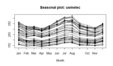
• A seasonality plot of US electricity usage
• A seasonal plot will show the data from each season overlapped
• A seasonal subseries plot is a specialized technique for showing seasonality
• Multiple box plots can be used as an alternative to the seasonal subseries plot to detect seasonality
• An autocorrelation plot (ACF) and a spectral plot can help identify seasonality.

A really good way to find periodicity, including seasonality, in any regular series of data is to remove any overall trend first and then to inspect time periodicity.

The run sequence plot is a recommended first step for analyzing any time series. Although seasonality can sometimes be indicated by this plot, seasonality is shown more clearly by the seasonal subseries plot or the box plot. The seasonal subseries plot does an excellent job of showing both the seasonal differences (between group patterns) and also the within-group patterns. The box plot shows the seasonal difference (between group patterns) quite well, but it does not show within group patterns. However, for large data sets, the box plot is usually easier to read than the seasonal subseries plot.

The seasonal plot, seasonal subseries plot, and the box plot all assume that the seasonal periods are known. In most cases, the analyst will in fact, know this. For example, for monthly data, the period is 12 since there are 12 months in a year. However, if the period is not known, the autocorrelation plot can help. If there is significant seasonality, the autocorrelation plot should show spikes at lags equal to the period. For example, for monthly data, if there is a seasonality effect, we would expect to see significant peaks at lag 12, 24, 36, and so on (although the intensity may decrease the further out we go).

An autocorrelation plot (ACF) can be used to identify seasonality, as it calculates the difference (residual amount) between a Y value and a lagged value of Y. The result gives some points where the two values are close together ( no seasonality ), but other points where there is a large discrepancy. These points indicate a level of seasonality in the data.

An ACF (autocorrelation) plot, of Australia beer consumption data.

Semiregular cyclic variations might be dealt with by spectral density estimation.

Calculation

Seasonal variation is measured in terms of an index, called a seasonal index. It is an average that can be used to compare an actual observation relative to what it would be if there were no seasonal variation. An index value is attached to each period of the time series within a year. This implies that if monthly data are considered there are 12 separate seasonal indices, one for each month. The following methods use seasonal indices to measure seasonal variations of a time-series data.

• Method of simple averages
• Ratio to trend method
• Ratio-to-moving-average method
• Link relatives method

Method of simple averages

The measurement of seasonal variation by using the ratio-to-moving-average method provides an index to measure the degree of the seasonal variation in a time series. The index is based on a mean of 100, with the degree of seasonality measured by variations away from the base. For example, if we observe the hotel rentals in a winter resort, we find that the winter quarter index is 124. The value 124 indicates that 124 percent of the average quarterly rental occur in winter. If the hotel management records 1436 rentals for the whole of last year, then the average quarterly rental would be 359= (1436/4). As the winter-quarter index is 124, we estimate the number of winter rentals as follows:

359*(124/100)=445;

Here, 359 is the average quarterly rental. 124 is the winter-quarter index. 445 the seasonalized winter-quarter rental.

This method is also called the percentage moving average method. In this method, the original data values in the time-series are expressed as percentages of moving averages. The steps and the tabulations are given below.

Ratio to trend method

1. Find the centered 12 monthly (or 4 quarterly) moving averages of the original data values in the time-series.

   
   

2. Express each original data value of the time-series as a percentage of the corresponding centered moving average values obtained in step(1). In other words, in a multiplicative time-series model, we get (Original data values) / (Trend values) × 100 = (T × C × S × I) / (T × C) × 100 = (S × I ) × 100.
   This implies that the ratio–to-moving average represents the seasonal and irregular components.

   
   

   
   

3. Arrange these percentages according to months or quarter of given years. Find the averages over all months or quarters of the given years.

   
   

4. If the sum of these indices is not 1200 (or 400 for quarterly figures), multiply then by a correction factor = 1200 / (sum of monthly indices). Otherwise, the 12 monthly averages will be considered as seasonal indices.

Ratio-to-moving-average method

Let us calculate the seasonal index by the ratio-to-moving-average method from the following data:

Sample Data

Year/Quarters	1	2	3	4
1996	75	60	54	59
1997	86	65	63	80
1998	90	72	66	85
1999	100	78	72	93

Now calculations for 4 quarterly moving averages and ratio-to-moving-averages are shown in the below table.

Moving Averages

Year	Quarter	Original Values(Y)	4 Figures Moving Total	4 Figures Moving Average	2 Figures Moving Total	2 Figures Moving Average(T)	Ratio-to-Moving-Average(%)(Y)/ (T)*100
1996	1	75			—	—	—
			—	—
	2	60			—	—	—
			248	62.00
	3	54			126.75	63.375	85.21
			259	64.75
	4	59			130.75	65.375	90.25
			264	66.00
1997	1	86			134.25	67.125	128.12
			273	68.25
	2	65			141.75	70.875	91.71
			294	73.50
	3	63			148.00	74.00	85.13
			298	74.50
	4	80			150.75	75.375	106.14
			305	76.25
1998	1	90			153.25	76.625	117.45
			308	77.00
	2	72			155.25	77.625	92.75
			313	78.25
	3	66			159.00	79.50	83.02
			323	80.75
	4	85			163.00	81.50	104.29
			329	82.25
1999	1	100			166.00	83.00	120.48
			335	83.75
	2	78			169.50	84.75	92.03
			343	85.75
	3	72			—	—	—
			—	—
	4	93			—	—	—

Calculation of Seasonal Index

Years/Quarters	1	2	3	4	Total
1996	—	—	85.21	90.25
1997	128.12	91.71	85.13	106.14
1998	117.45	92.75	83.02	104.29
1999	120.48	92.04	—	—
Total	366.05	276.49	253.36	300.68
Seasonal Average	122.01	92.16	84.45	100.23	398.85
Adjusted Seasonal Average	122.36	92.43	84.69	100.52	400

Now the total of seasonal averages is 398.85. Therefore, the corresponding correction factor would be 400/398.85 = 1.00288. Each seasonal average is multiplied by the correction factor 1.00288 to get the adjusted seasonal indices as shown in the above table.

Link relatives method

1. In an additive time-series model, the seasonal component is estimated as:

S = Y – (T + C + I )

where

S : Seasonal values

Y : Actual data values of the time-series

T : Trend values

C : Cyclical values

I : Irregular values.

2. In a multiplicative time-series model, the seasonal component is expressed in terms of ratio and percentage as

Seasonal effect ${\displaystyle ={\frac {T\cdot S\cdot C\cdot I}{T\cdot C\cdot I}}\times 100\ ={\frac {Y}{T\cdot C\cdot I}}\times 100}$;

However, in practice the detrending of time-series is done to arrive at ${\displaystyle S\cdot C\cdot I}$.

This is done by dividing both sides of ${\displaystyle Y=T\cdot S\cdot C\cdot I}$ by trend values T so that ${\displaystyle {\frac {Y}{T}}=S\cdot C\cdot I}$.

3. The deseasonalized time-series data will have only trend (T ), cyclical (C ) and irregular (I ) components and is expressed as:

• Multiplicative model : ${\displaystyle {\frac {Y}{S}}\times 100={\frac {T\cdot S\cdot C\cdot I}{S}}\times 100=(T\cdot C\cdot I)\times 100}$

• Additive model: Y – S = (T + S + C + I ) – S = T + C + I

Modeling

A completely regular cyclic variation in a time series might be dealt with in time series analysis by using a sinusoidal model with one or more sinusoids whose period-lengths may be known or unknown depending on the context. A less completely regular cyclic variation might be dealt with by using a special form of an ARIMA model which can be structured so as to treat cyclic variations semi-explicitly. Such models represent cyclostationary processes.

Another method of modelling periodic seasonality is the use of pairs of Fourier terms. Similar to using the sinusoidal model, Fourier terms added into regression models utilize sine and cosine terms in order to simulate seasonality. However, the seasonality of such a regression would be represented as the sum of sine or cosine terms, instead of a single sine or cosine term in a sinusoidal model. Every periodic function can be approximated with the inclusion of Fourier terms.

The difference between a sinusoidal model and a regression with Fourier terms can be simplified as below:

Sinusoidal Model:

${\displaystyle Y_{i}=a+bt+\alpha \sin(2\pi \omega T_{i}+\phi )+E_{i}}$

Regression With Fourier Terms:

${\displaystyle Y_{i}=a+bt+(\sum _{k=1}^{K}\alpha _{k}\cdot \sin({\tfrac {2\pi kt}{m}})+\beta _{k}\cdot \cos({\tfrac {2\pi kt}{n}}))+E_{i}}$

Seasonal adjustment

Main article: Seasonal adjustment

Seasonal adjustment or deseasonalization is any method for removing the seasonal component of a time series. The resulting seasonally adjusted data are used, for example, when analyzing or reporting non-seasonal trends over durations rather longer than the seasonal period. An appropriate method for seasonal adjustment is chosen on the basis of a particular view taken of the decomposition of time series into components designated with names such as "trend", "cyclic", "seasonal" and "irregular", including how these interact with each other. For example, such components might act additively or multiplicatively. Thus, if a seasonal component acts additively, the adjustment method has two stages:

• estimate the seasonal component of variation in the time series, usually in a form that has a zero mean across series;
• subtract the estimated seasonal component from the original time series, leaving the seasonally adjusted series: ${\displaystyle Y_{t}-S_{t}=T_{t}+E_{t}}$.

If it is a multiplicative model, the magnitude of the seasonal fluctuations will vary with the level, which is more likely to occur with economic series. When taking seasonality into account, the seasonally adjusted multiplicative decomposition can be written as ${\displaystyle Y_{t}/S_{t}=T_{t}*E_{t}}$; whereby the original time series is divided by the estimated seasonal component.

The multiplicative model can be transformed into an additive model by taking the log of the time series;

SA Multiplicative decomposition: ${\displaystyle Y_{t}=S_{t}*T_{t}*E_{t}}$

Taking log of the time series of the multiplicative model: ${\displaystyle logY_{t}=logS_{t}+logT_{t}+logE_{t}}$

One particular implementation of seasonal adjustment is provided by X-12-ARIMA.

In regression analysis

In regression analysis such as ordinary least squares, with a seasonally varying dependent variable being influenced by one or more independent variables, the seasonality can be accounted for and measured by including n-1 dummy variables, one for each of the seasons except for an arbitrarily chosen reference season, where n is the number of seasons (e.g., 4 in the case of meteorological seasons, 12 in the case of months, etc.). Each dummy variable is set to 1 if the data point is drawn from the dummy's specified season and 0 otherwise. Then the predicted value of the dependent variable for the reference season is computed from the rest of the regression, while for any other season it is computed using the rest of the regression and by inserting the value 1 for the dummy variable for that season.

Related patterns

It is important to distinguish seasonal patterns from related patterns. While a seasonal pattern occurs when a time series is affected by the season or the time of the year, such as annual, semiannual, quarterly, etc. A cyclic pattern, or simply a cycle, occurs when the data exhibit rises and falls in other periods, i.e., much longer (e.g., decadal) or much shorter (e.g., weekly) than seasonal. A quasiperiodicity is a more general, irregular periodicity.

Waste heat

From Wikipedia, the free encyclopedia

https://en.wikipedia.org/wiki/Waste_heat 

 

Thermal oxidizers can use a regenerative process for waste heat from industrial systems.

 

Air conditioning units extract heat from a dwelling interior with coolant, and transfer it to the dwelling exterior as waste. They emit additional heat in their use of electricity to power the devices that pass heat to and from the coolant

Waste heat is heat that is produced by a machine, or other process that uses energy, as a byproduct of doing work. All such processes give off some waste heat as a fundamental result of the laws of thermodynamics. Waste heat has lower utility (or in thermodynamics lexicon a lower exergy or higher entropy) than the original energy source. Sources of waste heat include all manner of human activities, natural systems, and all organisms, for example, incandescent light bulbs get hot, a refrigerator warms the room air, a building gets hot during peak hours, an internal combustion engine generates high-temperature exhaust gases, and electronic components get warm when in operation.

Instead of being "wasted" by release into the ambient environment, sometimes waste heat (or cold) can be used by another process (such as using hot engine coolant to heat a vehicle), or a portion of heat that would otherwise be wasted can be reused in the same process if make-up heat is added to the system (as with heat recovery ventilation in a building).

Thermal energy storage, which includes technologies both for short- and long-term retention of heat or cold, can create or improve the utility of waste heat (or cold). One example is waste heat from air conditioning machinery stored in a buffer tank to aid in night time heating. Another is seasonal thermal energy storage (STES) at a foundry in Sweden. The heat is stored in the bedrock surrounding a cluster of heat exchanger equipped boreholes, and is used for space heating in an adjacent factory as needed, even months later. An example of using STES to use natural waste heat is the Drake Landing Solar Community in Alberta, Canada, which, by using a cluster of boreholes in bedrock for interseasonal heat storage, obtains 97 percent of its year-round heat from solar thermal collectors on the garage roofs.Another STES application is storing winter cold underground, for summer air conditioning.

On a biological scale, all organisms reject waste heat as part of their metabolic processes, and will die if the ambient temperature is too high to allow this.

Anthropogenic waste heat is thought by some to contribute to the urban heat island effect. The biggest point sources of waste heat originate from machines (such as electrical generators or industrial processes, such as steel or glass production) and heat loss through building envelopes. The burning of transport fuels is a major contribution to waste heat.

Conversion of energy

See also: Second law of thermodynamics

Machines converting energy contained in fuels to mechanical work or electric energy produce heat as a by-product.

Sources

In the majority of energy applications, energy is required in multiple forms. These energy forms typically include some combination of: heating, ventilation, and air conditioning, mechanical energy and electric power. Often, these additional forms of energy are produced by a heat engine, running on a source of high-temperature heat. A heat engine can never have perfect efficiency, according to the second law of thermodynamics, therefore a heat engine will always produce a surplus of low-temperature heat. This is commonly referred to as waste heat or "secondary heat", or "low-grade heat". This heat is useful for the majority of heating applications, however, it is sometimes not practical to transport heat energy over long distances, unlike electricity or fuel energy. The largest proportions of total waste heat are from power stations and vehicle engines. The largest single sources are power stations and industrial plants such as oil refineries and steelmaking plants.

Power generation

The electrical efficiency of thermal power plants is defined as the ratio between the input and output energy. It is typically only 33% when disregarding usefulness of the heat output for building heat. The images show cooling towers which allow power stations to maintain the low side of the temperature difference essential for conversion of heat differences to other forms of energy. Discarded or "Waste" heat that is lost to the environment may instead be used to advantage.

Coal-fired power station that transform chemical energy into 36%-48% electricity and remaining 52%-64% to waste heat

Industrial processes

Industrial processes, such as oil refining, steel making or glass making are major sources of waste heat.

Electronics

Although small in terms of power, the disposal of waste heat from microchips and other electronic components, represents a significant engineering challenge. This necessitates the use of fans, heatsinks, etc. to dispose of the heat.

For example, data centers use electronic components that consume electricity for computing, storage and networking. The French CNRS explains a data center is like a resistor and most of the energy it consumes is transformed into heat and requires cooling systems.

Biological

Animals, including humans, create heat as a result of metabolism. In warm conditions, this heat exceeds a level required for homeostasis in warm-blooded animals, and is disposed of by various thermoregulation methods such as sweating and panting. Fiala et al. modelled human thermoregulation.

Cooling towers evaporating water at Ratcliffe-on-Soar Power Station, United Kingdom.

Disposal

Low temperature heat contains very little capacity to do work (Exergy), so the heat is qualified as waste heat and rejected to the environment. Economically most convenient is the rejection of such heat to water from a sea, lake or river. If sufficient cooling water is not available, the plant can be equipped with a cooling tower or air cooler to reject the waste heat into the atmosphere. In some cases it is possible to use waste heat, for instance in district heating systems.

Uses

Conversion to electricity

There are many different approaches to transfer thermal energy to electricity, and the technologies to do so have existed for several decades.

An established approach is by using a thermoelectric device, where a change in temperature across a semiconductor material creates a voltage through a phenomenon known as the Seebeck effect.

A related approach is the use of thermogalvanic cells, where a temperature difference gives rise to an electric current in an electrochemical cell.

The organic Rankine cycle, offered by companies such as Ormat, is a very known approach, whereby an organic substance is used as working medium instead of water. The benefit is that this process can reject heat at lower temperatures for the production of electricity than the regular water steam cycle. An example of use of the steam Rankine cycle is the Cyclone Waste Heat Engine.

Cogeneration and trigeneration

Waste of the by-product heat is reduced if a cogeneration system is used, also known as a Combined Heat and Power (CHP) system. Limitations to the use of by-product heat arise primarily from the engineering cost/efficiency challenges in effectively exploiting small temperature differences to generate other forms of energy. Applications utilizing waste heat include swimming pool heating and paper mills. In some cases, cooling can also be produced by the use of absorption refrigerators for example, in this case it's called trigeneration or CCHP (combined cooling, heat and power).

District heating

Waste heat can be used in district heating. Depending on the temperature of the waste heat and the district heating system, a heat pump must be used, to reach sufficient temperatures. An easy and cheap way to use waste heat in cold district heating systems, as these are operated at ambient temperatures and therefore even low-grade waste heat can be used without needing a heat pump at the producer side.

Pre-heating

Waste heat can be forced to heat incoming fluids and objects before being highly heated. For instance outgoing water can give its waste heat to incoming water in a heat exchanger before heating in homes or power plants.

Anthropogenic heat

Anthropogenic heat

Anthropogenic heat is heat generated by humans and human activity. The American Meteorological Society defines it as "Heat released to the atmosphere as a result of human activities, often involving combustion of fuels. Sources include industrial plants, space heating and cooling, human metabolism, and vehicle exhausts. In cities this source typically contributes 15–50 W/m² to the local heat balance, and several hundred W/m² in the center of large cities in cold climates and industrial areas."

Environmental impact

Anthropogenic heat is a small influence on rural temperatures, and becomes more significant in dense urban areas. It is one contributor to urban heat islands. Other human-caused effects (such as changes to albedo, or loss of evaporative cooling) that might contribute to urban heat islands are not considered to be anthropogenic heat by this definition.

Anthropogenic heat is a much smaller contributor to global warming than are greenhouse gases. In 2005, anthropogenic waste heat flux globally accounted for only 1% of the energy flux created by anthropogenic greenhouse gases. The heat flux is not evenly distributed, with some regions higher than others, and significantly higher in certain urban areas. For example, global forcing from waste heat in 2005 was 0.028 W/m², but was +0.39 and +0.68 W/m² for the continental United States and western Europe, respectively.

Although waste heat has been shown to have influence on regional climates, climate forcing from waste heat is not normally calculated in state-of-the-art global climate simulations. Equilibrium climate experiments show statistically significant continental-scale surface warming (0.4–0.9 °C) produced by one 2100 AHF scenario, but not by current or 2040 estimates. Simple global-scale estimates with different growth rates of anthropogenic heat that have been actualized recently show noticeable contributions to global warming, in the following centuries. For example, a 2% p.a. growth rate of waste heat resulted in a 3 degree increase as a lower limit for the year 2300. Meanwhile, this has been confirmed by more refined model calculations.

One research showed that if anthropogenic heat emissions continue to rise at the current rate, they will become a source of warming as strong as GHG emissions in the 21st century.

Thermography

From Wikipedia, the free encyclopedia

https://en.wikipedia.org/wiki/Thermography 

Thermogram of a traditional building in the background and a "passive house" in the foreground

Infrared thermography (IRT), thermal video and/or thermal imaging, is a process where a thermal camera captures and creates an image of an object by using infrared radiation emitted from the object in a process, which are examples of infrared imaging science. Thermographic cameras usually detect radiation in the long-infrared range of the electromagnetic spectrum (roughly 9,000–14,000 nanometers or 9–14 μm) and produce images of that radiation, called thermograms. Since infrared radiation is emitted by all objects with a temperature above absolute zero according to the black body radiation law, thermography makes it possible to see one's environment with or without visible illumination. The amount of radiation emitted by an object increases with temperature; therefore, thermography allows one to see variations in temperature. When viewed through a thermal imaging camera, warm objects stand out well against cooler backgrounds; humans and other warm-blooded animals become easily visible against the environment, day or night. As a result, thermography is particularly useful to the military and other users of surveillance cameras.

Thermogram of a cat

Some physiological changes in human beings and other warm-blooded animals can also be monitored with thermal imaging during clinical diagnostics. Thermography is used in allergy detection and veterinary medicine. Some alternative medicine practitioners promote its use for breast screening, despite the FDA warning that "those who opt for this method instead of mammography may miss the chance to detect cancer at its earliest stage". Government and airport personnel used thermography to detect suspected swine flu cases during the 2009 pandemic.

Thermal imaging camera and screen. Thermal imaging can detect elevated body temperature, one of the signs of the virus H1N1 (swine influenza).

Thermography has a long history, although its use has increased dramatically with the commercial and industrial applications of the past fifty years. Firefighters use thermography to see through smoke, to find persons, and to localize the base of a fire. Maintenance technicians use thermography to locate overheating joints and sections of power lines, which are a sign of impending failure. Building construction technicians can see thermal signatures that indicate heat leaks in faulty thermal insulation and can use the results to improve the efficiency of heating and air-conditioning units.

The appearance and operation of a modern thermographic camera is often similar to a camcorder. Often the live thermogram reveals temperature variations so clearly that a photograph is not necessary for analysis. A recording module is therefore not always built-in.

Specialized thermal imaging cameras use focal plane arrays (FPAs) that respond to longer wavelengths (mid- and long-wavelength infrared). The most common types are InSb, InGaAs, HgCdTe and QWIP FPA. The newest technologies use low-cost, uncooled microbolometers as FPA sensors. Their resolution is considerably lower than that of optical cameras, mostly 160x120 or 320x240 pixels, up to 1280 x 1024 for the most expensive models. Thermal imaging cameras are much more expensive than their visible-spectrum counterparts, and higher-end models are often export-restricted due to the military uses for this technology. Older bolometers or more sensitive models such as InSb require cryogenic cooling, usually by a miniature Stirling cycle refrigerator or liquid nitrogen.

Thermal energy

A comparison of a thermal image (top) and an ordinary photograph (bottom). The plastic bag is mostly transparent to long-wavelength infrared, but the man's glasses are opaque.

 

This thermogram shows excessive heating on a terminal in an industrial electrical fuse block.

Thermal images, or thermograms, are actually visual displays of the amount of infrared energy emitted, transmitted, and reflected by an object. Because there are multiple sources of the infrared energy, it is difficult to get an accurate temperature of an object using this method. A thermal imaging camera is capable of performing algorithms to interpret that data and build an image. Although the image shows the viewer an approximation of the temperature at which the object is operating, the camera is actually using multiple sources of data based on the areas surrounding the object to determine that value rather than detecting the actual temperature.

This phenomenon may become clearer upon consideration of the formula:

Incident Radiant Power = Emitted Radiant Power + Transmitted Radiant Power + Reflected Radiant Power;

where incident radiant power is the radiant power profile when viewed through a thermal imaging camera. Emitted radiant power is generally what is intended to be measured; transmitted radiant power is the radiant power that passes through the subject from a remote thermal source, and; reflected radiant power is the amount of radiant power that reflects off the surface of the object from a remote thermal source.

This phenomenon occurs everywhere, all the time. It is a process known as radiant heat exchange, since radiant power × time equals radiant energy. However, in the case of infrared thermography, the above equation is used to describe the radiant power within the spectral wavelength passband of the thermal imaging camera in use. The radiant heat exchange requirements described in the equation apply equally at every wavelength in the electromagnetic spectrum.

If the object is radiating at a higher temperature than its surroundings, then power transfer will be taking place and power will be radiating from warm to cold following the principle stated in the second law of thermodynamics. So if there is a cool area in the thermogram, that object will be absorbing the radiation emitted by the warm object.

The ability of objects to emit is called emissivity, to absorb radiation is called absorptivity. Under outdoor environments, convective cooling from wind may also need to be considered when trying to get an accurate temperature reading.

The thermal imaging camera would next employ a series of mathematical algorithms. Since the camera is only able to see the electromagnetic radiation that is impossible to detect with the human eye, it will build a picture in the viewer and record a visible picture, usually in a JPG format.

In order to perform the role of non-contact temperature recorder, the camera will change the temperature of the object being viewed with its emissivity setting.

Other algorithms can be used to affect the measurement, including the transmission ability of the transmitting medium (usually air) and the temperature of that transmitting medium. All these settings will affect the ultimate output for the temperature of the object being viewed.

This functionality makes the thermal imaging camera an excellent tool for the maintenance of electrical and mechanical systems in industry and commerce. By using the proper camera settings and by being careful when capturing the image, electrical systems can be scanned and problems can be found. Faults with steam traps in steam heating systems are easy to locate.

In the energy savings area, the thermal imaging camera can do more. Because it can see the effective radiation temperature of an object as well as what that object is radiating towards, it can help locate sources of thermal leaks and overheated regions as well.

Emissivity

Emissivity is a term that is often misunderstood and misused. It represents a material's ability to emit thermal radiation and is an optical property of matter.

Each material has a different emissivity, which may vary by temperature and infrared wavelength. For example, clean metal surfaces have emissivity that decreases at longer wavelengths; many dielectric materials, such as quartz (SiO₂), sapphire (Al₂O₃), calcium fluoride (CaF₂), etc. have emissivity that increases at longer wavelength; simple oxides, such as iron oxide (Fe₂O₃) display relatively flat emissivity in the infrared spectrum.

A material's emissivity can range from a theoretical 0.00 (completely not-emitting) to an equally theoretical 1.00 (completely emitting). An example of a substance with low emissivity would be silver, with an emissivity coefficient of .02. An example of a substance with high emissivity would be asphalt, with an emissivity coefficient of .98.

A black body is a theoretical object with an emissivity of 1 that radiates thermal radiation characteristic of its contact temperature. That is, if the contact temperature of a thermally uniform black body radiator were 50 °C (122 °F), the black body would emit thermal radiation characteristic of 50 °C (122 °F).

Thermogram of a snake held by a human

An ordinary object emits less infrared radiation than a theoretical black body. The fraction of its actual emission to the theoretical emission (of the black body) is its emissivity (or emissivity coefficient).

In order to make a temperature measurement of an object using an infrared imager, it is necessary to estimate or determine the object's emissivity. For quick work, a thermographer may refer to an emissivity table for a given type of object, and enter that value into the imager. The imager would then calculate the object's contact temperature based on the value entered from the table and the object's emission of infrared radiation as detected by the imager.

In order to get a more accurate temperature measurement, a thermographer may apply a standard material of known, high emissivity to the surface of the object. The standard material might be as complex as industrial emissivity spray produced specifically for the purpose, or as simple as standard black insulation tape, with an emissivity of about 0.97. The object's known temperature can then be measured using the standard emissivity. If desired, the object's actual emissivity (on a part of the object that is not covered by the standard material) can then be determined by adjusting the imager's setting to the known temperature. There are situations, however, when such an emissivity test is not possible due to dangerous or inaccessible conditions. In these situations, the thermographer must rely on tables.

Difference from infrared film

IR film is sensitive to infrared (IR) radiation in the 250 to 500 °C (482 to 932 °F) range, while the range of thermography is approximately −50 to 2,000 °C (−58 to 3,632 °F). So, for an IR film to work thermographically, it must be over 250 °C (482 °F) or be reflecting infrared radiation from something that is at least that hot.

Night vision infrared devices image in the near-infrared, just beyond the visual spectrum, and can see emitted or reflected near-infrared in complete visual darkness. However, again, these are not usually used for thermography due to the high temperature requirements, but are instead used with active near-IR sources.

Starlight-type night vision devices generally only magnify ambient light.

Passive vs. active thermography

All objects above the absolute zero temperature (0 K) emit infrared radiation. Hence, an excellent way to measure thermal variations is to use an infrared vision device, usually a focal plane array (FPA) infrared camera capable of detecting radiation in the mid (3 to 5 μm) and long (7 to 14 μm) wave infrared bands, denoted as MWIR and LWIR, corresponding to two of the high transmittance infrared windows. Abnormal temperature profiles at the surface of an object are an indication of a potential problem.

In passive thermography, the features of interest are naturally at a higher or lower temperature than the background. Passive thermography has many applications such as surveillance of people on a scene and medical diagnosis (specifically thermology).

In active thermography, an energy source is required to produce a thermal contrast between the feature of interest and the background. The active approach is necessary in many cases given that the inspected parts are usually in equilibrium with the surroundings. Given the super-linearities of the black-body radiation, active thermography can also be used to enhance the resolution of imaging systems beyond their diffraction limit or to achieve super-resolution microscopy.

Advantages

It shows a visual picture so temperatures over a large area can be compared. It is capable of catching moving targets in real time. It is able to find deterioration, i.e., higher temperature components prior to their failure. It can be used to measure or observe in areas inaccessible or hazardous for other methods. It is a non-destructive test method. It can be used to find defects in shafts, pipes, and other metal or plastic parts. It can be used to detect objects in dark areas. It has some medical application, essentially in physiotherapy.

Limitations and disadvantages

There are various cameras cheaper and more expensive. Quality cameras often have a high price range (often US$3,000 or more) due to the expense of the larger pixel array (state of the art 1280 x 1024), while less expensive models (with pixel arrays of 40x40 up to 160x120 pixels) are also available. Fewer pixels reduce the image quality making it more difficult to distinguish proximate targets within the same field of view.

There is also a difference in refresh rate. Some cameras may only have a refreshing value of 5 –15 Hz, other (e.g. FLIR X8500sc) 180 Hz or even more in no full window mode.

Also the lens can be integrated or not.

Many models do not provide the irradiance measurements used to construct the output image; the loss of this information without a correct calibration for emissivity, distance, and ambient temperature and relative humidity entails that the resultant images are inherently incorrect measurements of temperature.

Images can be difficult to interpret accurately when based upon certain objects, specifically objects with erratic temperatures, although this problem is reduced in active thermal imaging.

Thermographic cameras create thermal images based on the radiant heat energy it receives. As radiation levels are influenced by the emissivity and reflection of radiation such as sunlight from the surface being measured this causes errors in the measurements.

• Most cameras have ±2% accuracy or worse in measurement of temperature and are not as accurate as contact methods.
• Methods and instruments are limited to directly detecting surface temperatures.

If thermographic cameras or thermal sensors are used for aerial thermography or remote sensing, consideration should be given to the mounting method and position relative to the aircraft. If the aircraft's engine's exhaust is in proximity to the sensor, this can interfere with the sensor's ability to correctly capture ground radiation.

Applications

Kite aerial thermogram revealing features on/under a grassed playing field. Thermal inertia and differential transpiration/evaporation are involved

 

UAS thermal imagery of a solar panel array in Switzerland

 

AN/PAS-13 thermal rifle scope mounted on an AR-15 rifle

• Condition monitoring
• Low slope and flat roofing inspections
• Building diagnostics including building envelope inspections, moisture inspections, and energy losses in buildings
• Thermal mapping
• Digital infrared thermal imaging in health care
• Medical imaging
• Non-contact thermography, contact thermography and dynamic angiothermography
• Peripheral vascular disease screening.
• Carotid artery stenosis (CAS) screening through skin thermal maps.
• Active Dynamic Thermography (ADT) for medical applications.
• Neuromusculoskeletal disorders.
• Extracranial cerebral and facial vascular disease.
• Thyroid gland abnormalities.
• Various other neoplastic, metabolic, and inflammatory conditions.
• Archaeological kite aerial thermography
• Thermology
• Veterinary Thermal Imaging
• Night vision and Targeting
• UAV Surveillance
• Stereo vision
• Research
• Process control
• Nondestructive testing
• Surveillance in security, law enforcement and defence
• Chemical imaging
• Volcanology
• Building

Thermal imaging cameras convert the energy in the infrared wavelength into a visible light display. All objects above absolute zero emit thermal infrared energy, so thermal cameras can passively see all objects, regardless of ambient light. However, most thermal cameras only see objects warmer than −50 °C (−58 °F).

The spectrum and amount of thermal radiation depend strongly on an object's surface temperature. This makes it possible for a thermal imaging camera to display an object's temperature. However, other factors also influence the radiation, which limits the accuracy of this technique. For example, the radiation depends not only on the temperature of the object, but is also a function of the emissivity of the object. Also, radiation originates from the surroundings and is reflected in the object, and the radiation from the object and the reflected radiation will also be influenced by the absorption of the atmosphere.

Standards

ASTM International (ASTM)

• ASTM C1060, Standard Practice for Thermographic Inspection of Insulation Installations in Envelope Cavities of Frame Buildings
• ASTM C1153, Standard Practice for the Location of Wet Insulation in Roofing Systems Using Infrared Imaging
• ATSM D4788, Standard Test Method for Detecting Delamination in Bridge Decks Using Infrared Thermography
• ASTM E1186, Standard Practices for Air Leakage Site Detection in Building Envelopes and Air Barrier Systems
• ASTM E1934, Standard Guide for Examining Electrical and Mechanical Equipment with Infrared Thermography
• Standard for Infrared Inspection of Electrical Systems and Rotating Equipment
• Standard for Infrared Inspection of Insulated Roofs
• Standard for Infrared Inspection of Building Envelopes
• Standard for Infrared Inspections to Detect Pests and Pest Related Damage
• Standard for Infrared Inspection of Installed Photovoltaic (PV) Systems
• Standard for Infrared Inspection of Recreational Yachts and Small Craft Constructed of Fiberglass Reinforced Plastic and Composite Materials
• Standard for Infrared Thermal Imaging of Horses
• Standard for Measuring and Compensating for Emittance Using Infrared Imaging Radiometers
• Standard for Measuring and Compensating for Reflected Temperature Using Infrared Imaging Radiometers
• Standard for Measuring and Compensating for Transmittance of an Attenuating Medium Using Infrared Imaging Radiometers
• Standard for Measuring Distance/Target Size Values for Infrared Imaging Radiometers

International Organization for Standardization (ISO)

• ISO 6781, Thermal insulation – Qualitative detection of thermal irregularities in building envelopes – Infrared method
• ISO 18434-1, Condition monitoring and diagnostics of machines – Thermography – Part 1: General procedures
• ISO 18436-7, Condition monitoring and diagnostics of machines – Requirements for qualification and assessment of personnel – Part 7: Thermography

Biological counterpart

Thermography by definition is by means of an instrument (artifact), but some living creatures have natural organs that function as counterparts to bolometers, and thus possess a crude type of thermal imaging capability (thermoception). One of the best known examples is infrared sensing in snakes.

CCD and CMOS thermography

Color contours of temperature for a smoldering ember measured with a CMOS camera.

Non-specialized CCD and CMOS sensors have most of their spectral sensitivity in the visible light wavelength range. However, by utilizing the "trailing" area of their spectral sensitivity, namely the part of the infrared spectrum called near-infrared (NIR), and by using off-the-shelf CCTV camera it is possible under certain circumstances to obtain true thermal images of objects with temperatures at about 280 °C (536 °F) and higher.

At temperatures of 600 °C and above, inexpensive cameras with CCD and CMOS sensors have also been used for pyrometry in the visible spectrum. They have been used for soot in flames, burning coal particles, heated materials, SiC filaments, and smoldering embers. This pyrometry has been performed using external filters or only the sensor's Bayer filters. It has been performed using color ratios, grayscales, and/or a hybrid of both.