Flowering plant

From Wikipedia, the free encyclopedia

https://en.wikipedia.org/wiki/Flowering_plant 

Flowering plant Temporal range: Cretaceous (Late Valanginian) – present, 134–0 Ma PreꞒ Ꞓ O S D C P T J K Pg N
Diversity of angiosperms
Scientific classification
Kingdom:	Plantae
Clade:	Tracheophytes
Clade:	Spermatophytes
Clade:	Angiosperms
Groups (APG IV)
Basal angiosperms Amborellales Nymphaeales Austrobaileyales Core angiosperms Clades Magnoliids Monocots Eudicots Orders Chloranthales Ceratophyllales
Synonyms
Anthophyta Cronquist Angiospermae Lindl. Magnoliophyta Cronquist, Takht. & W.Zimm. Magnolicae Takht.

Flowering plants are plants that bear flowers and fruits, and form the clade Angiospermae (/ˌændʒiəˈspɜːrmiː/), commonly called angiosperms. The term "angiosperm" is derived from the Greek words angeion ('container, vessel') and sperma ('seed'), and refers to those plants that produce their seeds enclosed within a fruit. They are by far the most diverse group of land plants with 64 orders, 416 families, approximately 13,000 known genera and 300,000 known species. Angiosperms were formerly called Magnoliophyta (/mæɡˌnoʊliˈɒfətə, -əˈfaɪtə/).

Like gymnosperms, angiosperms are seed-producing plants. They are distinguished from gymnosperms by characteristics including flowers, endosperm within their seeds, and the production of fruits that contain the seeds.

The ancestors of flowering plants diverged from the common ancestor of all living gymnosperms before the end of the Carboniferous, over 300 million years ago. The closest fossil relatives of flowering plants are uncertain and contentious.

The earliest angiosperm fossils are in the form of pollen around 134 million years ago during the Early Cretaceous. Over the course of the Cretaceous, angiosperms explosively diversified, becoming the dominant group of plants across the planet by the end of the period, corresponding with the decline and extinction of previously widespread gymnosperm groups. The origin and diversification of the angiosperms is often known as "Darwin's abominable mystery".

Description

Chamaenerion angustifolium, also known as fireweed or rosebay willowherb, is a flowering plant in the willowherb family Onagraceae.

Angiosperm derived characteristics

Angiosperms differ from other seed plants in several ways, described in the table below. These distinguishing characteristics taken together have made the angiosperms the most diverse and numerous land plants, and the most commercially important group to humans.

Distinctive features of angiosperms

Feature	Description
Flowering organs	Flowers, the reproductive organs of flowering plants, are the most remarkable feature distinguishing them from the other seed plants. Flowers provided angiosperms with the means to have a more species-specific breeding system, and hence a way to evolve more readily into different species without the risk of crossing back with related species. Faster speciation enabled the angiosperms to adapt to a wider range of ecological niches. This has allowed flowering plants to largely dominate terrestrial ecosystems, comprising about 90 percent of all plant species.
Stamens with two pairs of pollen sacs	Stamens are much lighter than the corresponding organs of gymnosperms and have contributed to the diversification of angiosperms through time with adaptations to specialised pollination syndromes, such as particular pollinators. Stamens have also become modified through time to prevent self-fertilization, which has permitted further diversification, allowing angiosperms eventually to fill more niches.
Reduced male gametophyte, three cells	The male gametophyte in angiosperms is significantly reduced in size compared to those of gymnosperm seed plants. The smaller size of the pollen reduces the amount of time between pollination (the pollen grain reaching the female plant) and fertilization. In gymnosperms, fertilization can occur up to a year after pollination, whereas in angiosperms, fertilization begins very soon after pollination. The shorter amount of time between pollination and fertilization allows angiosperms to produce seeds earlier after pollination than gymnosperms, providing angiosperms a distinct evolutionary advantage.
Closed carpel enclosing the ovules (carpel or carpels and accessory parts may become the fruit)	The closed carpel of angiosperms also allows adaptations to specialised pollination syndromes and controls. This helps to prevent self-fertilization, thereby maintaining increased diversity. Once the ovary is fertilised, the carpel and some surrounding tissues develop into a fruit. This fruit often serves as an attractant to seed-dispersing animals. The resulting cooperative relationship presents another advantage to angiosperms in the process of dispersal.
Reduced female gametophyte, seven cells with eight nuclei	The reduced female gametophyte, like the reduced male gametophyte, may be an adaptation allowing for more rapid seed set, eventually leading to such flowering plant adaptations as annual herbaceous life-cycles, allowing the flowering plants to fill even more niches.
Endosperm	In general, endosperm formation begins after fertilization and before the first division of the zygote. Endosperm is a highly nutritive tissue that can provide food for the developing embryo, the cotyledons, and sometimes the seedling when it first appears.

Vascular anatomy

Cross-section of a stem of the angiosperm flax:
1. pith, 2. protoxylem, 3. xylem, 4. phloem, 5. sclerenchyma (bast fibre), 6. cortex, 7. epidermis

Angiosperm stems are made up of seven layers as shown on the right. The amount and complexity of tissue-formation in flowering plants exceeds that of gymnosperms.

In the dicotyledons, the vascular bundles of the stem are arranged such that the xylem and phloem form concentric rings. The bundles in the very young stem are arranged in an open ring, separating a central pith from an outer cortex. In each bundle, separating the xylem and phloem, is a layer of meristem or active formative tissue known as cambium. By the formation of a layer of cambium between the bundles (interfascicular cambium), a complete ring is formed, and a regular periodical increase in thickness results from the development of xylem on the inside and phloem on the outside. The soft phloem becomes crushed, but the hard wood persists and forms the bulk of the stem and branches of the woody perennial. Owing to differences in the character of the elements produced at the beginning and end of the season, the wood is marked out in transverse section into concentric rings, one for each season of growth, called annual rings.

Among the monocotyledons, the bundles are more numerous in the young stem and are scattered through the ground tissue. They contain no cambium and once formed the stem increases in diameter only in exceptional cases.

Reproductive anatomy

Main articles: Flower and Plant reproductive morphology

 

A collection of flowers forming an inflorescence.

The characteristic feature of angiosperms is the flower. Flowers show remarkable variation in form and elaboration, and provide the most trustworthy external characteristics for establishing relationships among angiosperm species. The function of the flower is to ensure fertilization of the ovule and development of fruit containing seeds. The floral apparatus may arise terminally on a shoot or from the axil of a leaf (where the petiole attaches to the stem). Occasionally, as in violets, a flower arises singly in the axil of an ordinary foliage-leaf. More typically, the flower-bearing portion of the plant is sharply distinguished from the foliage-bearing or vegetative portion, and forms a more or less elaborate branch-system called an inflorescence.

There are two kinds of reproductive cells produced by flowers. Microspores, which will divide to become pollen grains, are the "male" cells and are borne in the stamens (or microsporophylls). The "female" cells called megaspores, which will divide to become the egg cell (megagametogenesis), are contained in the ovule and enclosed in the carpel (or megasporophyll).

The flower may consist only of these parts, as in willow, where each flower comprises only a few stamens or two carpels. Usually, other structures are present and serve to protect the sporophylls and to form an envelope attractive to pollinators. The individual members of these surrounding structures are known as sepals and petals (or tepals in flowers such as Magnolia where sepals and petals are not distinguishable from each other). The outer series (calyx of sepals) is usually green and leaf-like, and functions to protect the rest of the flower, especially the bud. The inner series (corolla of petals) is, in general, white or brightly colored, and is more delicate in structure. It functions to attract insect or bird pollinators. Attraction is effected by color, scent, and nectar, which may be secreted in some part of the flower. The characteristics that attract pollinators account for the popularity of flowers and flowering plants among humans.

While the majority of flowers are perfect or hermaphrodite (having both pollen and ovule producing parts in the same flower structure), flowering plants have developed numerous morphological and physiological mechanisms to reduce or prevent self-fertilization. Heteromorphic flowers have short carpels and long stamens, or vice versa, so animal pollinators cannot easily transfer pollen to the pistil (receptive part of the carpel). Homomorphic flowers may employ a biochemical (physiological) mechanism called self-incompatibility to discriminate between self and non-self pollen grains. Alternatively, in dioecious species, the male and female parts are morphologically separated, developing on different individual flowers.

Taxonomy

History of classification

From 1736, an illustration of Linnaean classification

The botanical term "angiosperm", from Greek words angeíon (ἀγγεῖον 'bottle, vessel') and spérma (σπέρμα 'seed'), was coined in the form "Angiospermae" by Paul Hermann in 1690 but he used this term to refer to a group of plants which form only a subset of what today are known as angiosperms. Hermannn's Angiospermae including only flowering plants possessing seeds enclosed in capsules, distinguished from his Gymnospermae, which were flowering plants with achenial or schizo-carpic fruits, the whole fruit or each of its pieces being here regarded as a seed and naked. The terms Angiospermae and Gymnospermae were used by Carl Linnaeus with the same sense, but with restricted application, in the names of the orders of his class Didynamia.

The terms angiosperms and gymnosperm fundamentally changed in meaning in 1827 when Robert Brown established the existence of truly naked ovules in the Cycadeae and Coniferae. The term gymnosperm was from then on applied to seed plants with naked ovules, and the term angiosperm to seed plants with enclosed ovules. However, for many years after Brown's discovery, the primary division of the seed plants was seen as between monocots and dicots, with gymnosperms as a small subset of the dicots.

An auxanometer, a device for measuring increase or rate of growth in plants

In 1851, Hofmeister discovered the changes occurring in the embryo-sac of flowering plants, and determined the correct relationships of these to the Cryptogamia. This fixed the position of Gymnosperms as a class distinct from Dicotyledons, and the term Angiosperm then gradually came to be accepted as the suitable designation for the whole of the flowering plants other than Gymnosperms, including the classes of Dicotyledons and Monocotyledons. This is the sense in which the term is used today.

In most taxonomies, the flowering plants are treated as a coherent group. The most popular descriptive name has been Angiospermae, with Anthophyta (lit. 'flower-plants') a second choice (both unranked). The Wettstein system and Engler system treated them as a subdivision (Angiospermae). The Reveal system also treated them as a subdivision (Magnoliophytina), but later split it to Magnoliopsida, Liliopsida, and Rosopsida. The Takhtajan system and Cronquist system treat them as a division (Magnoliophyta). The Dahlgren system and Thorne system (1992) treat them as a class (Magnoliopsida). The APG system of 1998, and the later 2003 and 2009 revisions, treat the flowering plants as an unranked clade without a formal Latin name (angiosperms). A formal classification was published alongside the 2009 revision in which the flowering plants rank as a subclass (Magnoliidae).

The internal classification of this group has undergone considerable revision. The Cronquist system, proposed by Arthur Cronquist in 1968 and published in its full form in 1981, is still widely used but is no longer believed to accurately reflect phylogeny. A consensus about how the flowering plants should be arranged has recently begun to emerge through the work of the Angiosperm Phylogeny Group (APG), which published an influential reclassification of the angiosperms in 1998. Updates incorporating more recent research were published as the APG II system in 2003, the APG III system in 2009, and the APG IV system in 2016.

Traditionally, the flowering plants are divided into two groups,

• Dicotyledoneae or Magnoliopsida
• Monocotyledoneae or Liliopsida

to which the Cronquist system ascribes the classes Magnoliopsida (from "Magnoliaceae") and Liliopsida (from "Liliaceae"). Other descriptive names allowed by Article 16 of the ICBN include Dicotyledones or Dicotyledoneae, and Monocotyledones or Monocotyledoneae, which have a long history of use. In plain English, their members may be called "dicotyledons" ("dicots") and "monocotyledons" ("monocots"). The Latin behind these names refers the observation that the dicots most often have two cotyledons, or embryonic leaves, within each seed. The monocots usually have only one, but the rule is not absolute either way. From a broad diagnostic point of view, the number of cotyledons is neither a particularly handy, nor a reliable character.

Recent studies, as by the APG, show that the monocots form a monophyletic group (a clade) but that the dicots are paraphyletic. Nevertheless, the majority of dicot species fall into a clade, the eudicots or tricolpates, and most of the remaining fall into another major clade, the magnoliids, containing about 9,000 species. The rest include a paraphyletic grouping of early branching taxa known collectively as the basal angiosperms, plus the families Ceratophyllaceae and Chloranthaceae.

Modern classification

Monocot (left) and dicot seedlings

There are eight groups of living angiosperms:

• Basal angiosperms (ANA: Amborella, Nymphaeales, Austrobaileyales)
  • Amborella, a single species of shrub from New Caledonia;
  • Nymphaeales, about 80 species, water lilies and Hydatellaceae;
  • Austrobaileyales, about 100 species of woody plants from various parts of the world
• Core angiosperms (Mesangiospermae)
  • Chloranthales, 77 known species of aromatic plants with toothed leaves;
  • Magnoliids, about 10,000 species, characterised by trimerous flowers, pollen with one pore, and usually branching-veined leaves—for example magnolias, bay laurel, and black pepper;
  • Monocots, about 70,000 species, characterised by trimerous flowers, a single cotyledon, pollen with one pore, and usually parallel-veined leaves—for example grasses, orchids, and palms;
  • Ceratophyllum, about 6 species of aquatic plants, perhaps most familiar as aquarium plants;
  • Eudicots, about 175,000 species, characterised by 4- or 5-merous flowers, pollen with three pores, and usually branching-veined leaves—for example sunflowers, petunia, buttercup, apples, and oaks.

The exact relationships among these eight groups is not yet clear, although there is agreement that the first three groups to diverge from the ancestral angiosperm were Amborellales, Nymphaeales, and Austrobaileyales (basal angiosperms) Of the remaining five groups (core angiosperms), the relationships among the three broadest groups remains unclear (magnoliids, monocots, and eudicots). Zeng and colleagues (Fig. 1) describe four competing schemes.The eudicots and monocots are the largest and most diversified, with ~ 75% and 20% of angiosperm species, respectively. Some analyses make the magnoliids the first to diverge, others the monocots. Ceratophyllum seems to group with the eudicots rather than with the monocots. The APG IV retained the overall higher order relationship described in APG III.

Evolutionary history

Further information: Evolutionary history of plants § Flowers

Paleozoic

Fossilised spores suggest that land plants (embryophytes) have existed for at least 475 million years. Early land plants reproduced sexually with flagellated, swimming sperm, like the green algae from which they evolved. An adaptation to terrestrialization was the development of upright sporangia for dispersal by spores to new habitats. This feature is lacking in the descendants of their nearest algal relatives, the Charophycean green algae. A later terrestrial adaptation took place with retention of the delicate, avascular sexual stage, the gametophyte, within the tissues of the vascular sporophyte. This occurred by spore germination within sporangia rather than spore release, as in non-seed plants. A current example of how this might have happened can be seen in the precocious spore germination in Selaginella, the spike-moss. The result for the ancestors of angiosperms and gymnosperms was enclosing the female gamete in a case, the seed. The first seed bearing plants were gymnosperms, like the ginkgo, and conifers (such as pines and firs). These did not produce flowers. The pollen grains (male gametophytes) of Ginkgo and cycads produce a pair of flagellated, mobile sperm cells that "swim" down the developing pollen tube to the female and her eggs.

Angiosperms appear suddenly and in great diversity in the fossil record in the Early Cretaceous. This poses such a problem for the theory of gradual evolution that Charles Darwin called it an "abominable mystery". Several groups of extinct gymnosperms, in particular seed ferns, have been proposed as the ancestors of flowering plants, but there is no continuous fossil evidence showing how flowers evolved, and botanists still regard it as a mystery.

Several claims of pre-Cretaceous angiosperm fossils have been made, such as the upper Triassic Sanmiguelia lewisi, but none of these are widely accepted by paleobotanists. Oleanane, a secondary metabolite produced by many flowering plants, has been found in Permian deposits of that age together with fossils of gigantopterids. Gigantopterids are a group of extinct seed plants that share many morphological traits with flowering plants, although they are not known to have been flowering plants themselves. Molecular evidence suggests that the ancestors of angiosperms diverged from the gymnosperms during the late Devonian, about 365 million years ago, despite only appearing in the fossil record during the Early Cretaceous, almost two hundred million years later.

Triassic and Jurassic

Fluffy flowers of Tetradenia riparia (misty plume bush)

 

Flowers of Malus sylvestris (crab apple)

 

Flowers and leaves of Senecio angulatus (creeping groundsel)

 

Two bees on the composite flower head of creeping thistle, Cirsium arvense

Based on fossil evidence, some have proposed that the ancestors of the angiosperms diverged from an unknown group of gymnosperms in the Triassic period (245–202 million years ago). Fossil angiosperm-like pollen from the Middle Triassic (247.2–242.0 Ma) suggests an older date for their origin, which is further supported by genetic evidence of the ancestors of angiosperms diverging during the Devonian. A close relationship between angiosperms and gnetophytes, proposed on the basis of morphological evidence, has more recently been disputed on the basis of molecular evidence that suggest gnetophytes are instead more closely related to conifers and other gymnosperms.

The fossil plant species Nanjinganthus dendrostyla from Early Jurassic China seems to share many exclusively angiosperm features, such as a thickened receptacle with ovules, and thus might represent a crown-group or a stem-group angiosperm. However, these have been disputed by other researchers, who contend that the structures are misinterpreted decomposed conifer cones.

The evolution of seed plants and later angiosperms appears to be the result of two distinct rounds of whole genome duplication events. These occurred at 319 million years ago and 192 million years ago. Another possible whole genome duplication event at 160 million years ago perhaps created the ancestral line that led to all modern flowering plants. That event was studied by sequencing the genome of an ancient flowering plant, Amborella trichopoda.

One study has suggested that the early-middle Jurassic plant Schmeissneria, traditionally considered a type of ginkgo, may be the earliest known angiosperm, or at least a close relative. This, along with all other pre-Cretaceous angiosperm fossil claims, is strongly disputed by many paleobotanists.

Many paleobotanists consider the Caytoniales, a group of "seed ferns" that first appeared during the Triassic and went extinct in the Cretaceous, to be amongst the best candidates for a close relative of angiosperms.

Cretaceous

Whereas the earth had previously been dominated by ferns and conifers, angiosperms quickly spread during the Cretaceous. They now comprise about 90% of all plant species including most food crops. It has been proposed that the swift rise of angiosperms to dominance was facilitated by a reduction in their genome size. During the early Cretaceous period, only angiosperms underwent rapid genome downsizing, while genome sizes of ferns and gymnosperms remained unchanged. Smaller genomes—and smaller nuclei—allow for faster rates of cell division and smaller cells. Thus, species with smaller genomes can pack more, smaller cells—in particular veins and stomata—into a given leaf volume. Genome downsizing therefore facilitated higher rates of leaf gas exchange (transpiration and photosynthesis) and faster rates of growth. This would have countered some of the negative physiological effects of genome duplications, facilitated increased uptake of carbon dioxide despite concurrent declines in atmospheric CO₂ concentrations, and allowed the flowering plants to outcompete other land plants.

The oldest known fossils definitively attributable to angiosperms are reticulated monosulcate pollen from the late Valanginian (Early or Lower Cretaceous - 140 to 133 million years ago) of Italy and Israel, likely representative of the basal angiosperm grade.

The earliest known macrofossil confidently identified as an angiosperm, Archaefructus liaoningensis, is dated to about 125 million years BP (the Cretaceous period), whereas pollen considered to be of angiosperm origin takes the fossil record back to about 130 million years BP, with Montsechia representing the earliest flower at that time.

In 2013 flowers encased in amber were found and dated 100 million years before present. The amber had frozen the act of sexual reproduction in the process of taking place. Microscopic images showed tubes growing out of pollen and penetrating the flower's stigma. The pollen was sticky, suggesting it was carried by insects. In August 2017, scientists presented a detailed description and 3D model image of what the first flower possibly looked like, and presented the hypothesis that it may have lived about 140 million years ago. A Bayesian analysis of 52 angiosperm taxa suggested that the crown group of angiosperms evolved between 178 million years ago and 198 million years ago.

Recent DNA analysis based on molecular systematics showed that Amborella trichopoda, found on the Pacific island of New Caledonia, belongs to a sister group of the other flowering plants, and morphological studies suggest that it has features that may have been characteristic of the earliest flowering plants. The orders Amborellales, Nymphaeales, and Austrobaileyales diverged as separate lineages from the remaining angiosperm clade at a very early stage in flowering plant evolution.

The great angiosperm radiation, when a great diversity of angiosperms appears in the fossil record, occurred in the mid-Cretaceous (approximately 100 million years ago). However, a study in 2007 estimated that the division of the five most recent of the eight main groups occurred around 140 million years ago. (the genus Ceratophyllum, the family Chloranthaceae, the eudicots, the magnoliids, and the monocots) .

It is generally assumed that the function of flowers, from the start, was to involve mobile animals in their reproduction processes. That is, pollen can be scattered even if the flower is not brightly colored or oddly shaped in a way that attracts animals; however, by expending the energy required to create such traits, angiosperms can enlist the aid of animals and, thus, reproduce more efficiently.

Island genetics provides one proposed explanation for the sudden, fully developed appearance of flowering plants. Island genetics is believed to be a common source of speciation in general, especially when it comes to radical adaptations that seem to have required inferior transitional forms. Flowering plants may have evolved in an isolated setting like an island or island chain, where the plants bearing them were able to develop a highly specialised relationship with some specific animal (a wasp, for example). Such a relationship, with a hypothetical wasp carrying pollen from one plant to another much the way fig wasps do today, could result in the development of a high degree of specialisation in both the plant(s) and their partners. Note that the wasp example is not incidental; bees, which, it is postulated, evolved specifically due to mutualistic plant relationships, are descended from wasps.

Animals are also involved in the distribution of seeds. Fruit, which is formed by the enlargement of flower parts, is frequently a seed-dispersal tool that attracts animals to eat or otherwise disturb it, incidentally scattering the seeds it contains (see frugivory). Although many such mutualistic relationships remain too fragile to survive competition and to spread widely, flowering proved to be an unusually effective means of reproduction, spreading (whatever its origin) to become the dominant form of land plant life.

Flower ontogeny uses a combination of genes normally responsible for forming new shoots. The most primitive flowers probably had a variable number of flower parts, often separate from (but in contact with) each other. The flowers tended to grow in a spiral pattern, to be bisexual (in plants, this means both male and female parts on the same flower), and to be dominated by the ovary (female part). As flowers evolved, some variations developed parts fused together, with a much more specific number and design, and with either specific sexes per flower or plant or at least "ovary-inferior". Flower evolution continues to the present day; modern flowers have been so profoundly influenced by humans that some of them cannot be pollinated in nature. Many modern domesticated flower species were formerly simple weeds, which sprouted only when the ground was disturbed. Some of them tended to grow with human crops, perhaps already having symbiotic companion plant relationships with them, and the prettiest did not get plucked because of their beauty, developing a dependence upon and special adaptation to human affection.

A few paleontologists have also proposed that flowering plants, or angiosperms, might have evolved due to interactions with dinosaurs. One of the idea's strongest proponents is Robert T. Bakker. He proposes that herbivorous dinosaurs, with their eating habits, provided a selective pressure on plants, for which adaptations either succeeded in deterring or coping with predation by herbivores.

By the late Cretaceous, angiosperms appear to have dominated environments formerly occupied by ferns and cycadophytes, but large canopy-forming trees replaced conifers as the dominant trees only close to the end of the Cretaceous 66 million years ago or even later, at the beginning of the Paleogene. The radiation of herbaceous angiosperms occurred much later. Yet, many fossil plants recognisable as belonging to modern families (including beech, oak, maple, and magnolia) had already appeared by the late Cretaceous. Flowering plants appeared in Australia about 126 million years ago. This also pushed the age of ancient Australian vertebrates, in what was then a south polar continent, to 126-110 million years old.

Gallery of photos

• 

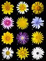
  A poster of twelve different species of flowers of the family Asteraceae

• 

  Lupinus pilosus

• 

  Bud of a pink rose

Diversity

The number of species of flowering plants is estimated to be in the range of 250,000 to 400,000. This compares to around 12,000 species of moss and 11,000 species of pteridophytes, showing that flowering plants are much more diverse. The number of families in APG (1998) was 462. In APG II (2003) it is not settled; at maximum it is 457, but within this number there are 55 optional segregates, so that the minimum number of families in this system is 402. In APG III (2009) there are 415 families. Compared to the APG III system, the APG IV system recognizes five new orders (Boraginales, Dilleniales, Icacinales, Metteniusales and Vahliales), along with some new families, making a total of 64 angiosperm orders and 416 families. The diversity of flowering plants is not evenly distributed. Nearly all species belong to the eudicot (75%), monocot (23%), and magnoliid (2%) clades. The remaining five clades contain a little over 250 species in total; i.e. less than 0.1% of flowering plant diversity, divided among nine families. The 43 most diverse of 443 families of flowering plants by species, in their APG circumscriptions, are

1. Asteraceae or Compositae (daisy family): 22,750 species;
2. Orchidaceae (orchid family): 21,950;
3. Fabaceae or Leguminosae (bean family): 19,400;
4. Rubiaceae (madder family): 13,150;
5. Poaceae or Gramineae (grass family): 10,035;
6. Lamiaceae or Labiatae (mint family): 7,175;
7. Euphorbiaceae (spurge family): 5,735;
8. Melastomataceae or Melastomaceae (melastome family): 5,005;
9. Myrtaceae (myrtle family): 4,625;
10. Apocynaceae (dogbane family): 4,555;
11. Cyperaceae (sedge family): 4,350;
12. Malvaceae (mallow family): 4,225;
13. Araceae (arum family): 4,025;
14. Ericaceae (heath family): 3,995;
15. Gesneriaceae (gesneriad family): 3,870;
16. Apiaceae or Umbelliferae (parsley family): 3,780;
17. Brassicaceae or Cruciferae (cabbage family): 3,710:
18. Piperaceae (pepper family): 3,600;
19. Bromeliaceae (bromeliad family): 3,540;
20. Acanthaceae (acanthus family): 3,500;
21. Rosaceae (rose family): 2,830;
22. Boraginaceae (borage family): 2,740;
23. Urticaceae (nettle family): 2,625;
24. Ranunculaceae (buttercup family): 2,525;
25. Lauraceae (laurel family): 2,500;
26. Solanaceae (nightshade family): 2,460;
27. Campanulaceae (bellflower family): 2,380;
28. Arecaceae (palm family): 2,361;
29. Annonaceae (custard apple family): 2,220;
30. Caryophyllaceae (pink family): 2,200;
31. Orobanchaceae (broomrape family): 2,060;
32. Amaranthaceae (amaranth family): 2,050;
33. Iridaceae (iris family): 2,025;
34. Aizoaceae or Ficoidaceae (ice plant family): 2,020;
35. Rutaceae (rue family): 1,815;
36. Phyllanthaceae (phyllanthus family): 1,745;
37. Scrophulariaceae (figwort family): 1,700;
38. Gentianaceae (gentian family): 1,650;
39. Convolvulaceae (bindweed family): 1,600;
40. Proteaceae (protea family): 1,600;
41. Sapindaceae (soapberry family): 1,580;
42. Cactaceae (cactus family): 1,500;
43. Araliaceae (Aralia or ivy family): 1,450.

Of these, the Orchidaceae, Poaceae, Cyperaceae, Araceae, Bromeliaceae, Arecaceae, and Iridaceae are monocot families; Piperaceae, Lauraceae, and Annonaceae are magnoliid dicots; the rest of the families are eudicots.

Reproduction

Fertilisation and embryogenesis

Main articles: Fertilization and Plant embryogenesis

 

Angiosperm life cycle

Double fertilization refers to a process in which two sperm cells fertilise cells in the ovule. This process begins when a pollen grain adheres to the stigma of the pistil (female reproductive structure), germinates, and grows a long pollen tube. While this pollen tube is growing, a haploid generative cell travels down the tube behind the tube nucleus. The generative cell divides by mitosis to produce two haploid (n) sperm cells. As the pollen tube grows, it makes its way from the stigma, down the style and into the ovary. Here the pollen tube reaches the micropyle of the ovule and digests its way into one of the synergids, releasing its contents (which include the sperm cells). The synergid that the cells were released into degenerates and one sperm makes its way to fertilise the egg cell, producing a diploid (2n) zygote. The second sperm cell fuses with both central cell nuclei, producing a triploid (3n) cell. As the zygote develops into an embryo, the triploid cell develops into the endosperm, which serves as the embryo's food supply. The ovary will now develop into a fruit and the ovule will develop into a seed.

Fruit and seed

Main articles: Seed and Fruit

 

The fruit of Aesculus hippocastanum, the horse chestnut tree

As the development of the embryo and endosperm proceeds within the embryo sac, the sac wall enlarges and combines with the nucellus (which is likewise enlarging) and the integument to form the seed coat. The ovary wall develops to form the fruit or pericarp, whose form is closely associated with type of seed dispersal system.

Frequently, the influence of fertilisation is felt beyond the ovary, and other parts of the flower take part in the formation of the fruit, e.g., the floral receptacle in the apple, strawberry, and others.

The character of the seed coat bears a definite relation to that of the fruit. They protect the embryo and aid in dissemination; they may also directly promote germination. Among plants with indehiscent fruits, in general, the fruit provides protection for the embryo and secures dissemination. In this case, the seed coat is only slightly developed. If the fruit is dehiscent and the seed is exposed, in general, the seed-coat is well developed and must discharge the functions otherwise executed by the fruit.

In some cases, like in the Asteraceae family, species have evolved to exhibit heterocarpy, or the production of different fruit morphs. These fruit morphs, produced from one plant, are different in size and shape, which influence dispersal range and germination rate. These fruit morphs are adapted to different environments, increasing chances for survival.

Meiosis

Like all diploid multicellular organisms that use sexual reproduction, flowering plants generate gametes using a specialised type of cell division called meiosis. Meiosis takes place in the ovule—a structure within the ovary that is located within the pistil at the centre of the flower (see diagram labeled "Angiosperm lifecycle"). A diploid cell (megaspore mother cell) in the ovule undergoes meiosis (involving two successive cell divisions) to produce four cells (megaspores) with haploid nuclei. It is thought that the basal chromosome number in angiosperms is n = 7. One of these four cells (megaspore) then undergoes three successive mitotic divisions to produce an immature embryo sac (megagametophyte) with eight haploid nuclei. Next, these nuclei are segregated into separate cells by cytokinesis to produce three antipodal cells, two synergid cells and an egg cell. Two polar nuclei are left in the central cell of the embryo sac.

Pollen is also produced by meiosis in the male anther (microsporangium). During meiosis, a diploid microspore mother cell undergoes two successive meiotic divisions to produce four haploid cells (microspores or male gametes). Each of these microspores, after further mitoses, becomes a pollen grain (microgametophyte) containing two haploid generative (sperm) cells and a tube nucleus. When a pollen grain makes contact with the female stigma, the pollen grain forms a pollen tube that grows down the style into the ovary. In the act of fertilisation, a male sperm nucleus fuses with the female egg nucleus to form a diploid zygote that can then develop into an embryo within the newly forming seed. Upon germination of the seed, a new plant can grow and mature.

The adaptive function of meiosis is currently a matter of debate. A key event during meiosis in a diploid cell is the pairing of homologous chromosomes and homologous recombination (the exchange of genetic information) between homologous chromosomes. This process promotes the production of increased genetic diversity among progeny and the recombinational repair of damages in the DNA to be passed on to progeny. To explain the adaptive function of meiosis in flowering plants, some authors emphasise diversity and others emphasise DNA repair.

Apomixis

Apomixis (reproduction via asexually formed seeds) is found naturally in about 2.2% of angiosperm genera. One type of apomixis, gametophytic apomixis found in a dandelion species involves formation of an unreduced embryo sac due to incomplete meiosis (apomeiosis) and development of an embryo from the unreduced egg inside the embryo sac, without fertilisation (parthenogenesis).

Some angiosperms, including many citrus varieties, are able to produce fruits through a type of apomixis called nucellar embryony.

Uses

Agriculture is almost entirely dependent on angiosperms, which provide virtually all plant-based food, and also provide a significant amount of livestock feed. Of all the families of plants, the Poaceae, or grass family (providing grains), is by far the most important, providing the bulk of all feedstocks (rice, maize, wheat, barley, rye, oats, pearl millet, sugar cane, sorghum). The Fabaceae, or legume family, comes in second place. Also of high importance are the Solanaceae, or nightshade family (potatoes, tomatoes, and peppers, among others); the Cucurbitaceae, or gourd family (including pumpkins and melons); the Brassicaceae, or mustard plant family (including rapeseed and the innumerable varieties of the cabbage species Brassica oleracea); and the Apiaceae, or parsley family. Many of our fruits come from the Rutaceae, or rue family (including oranges, lemons, grapefruits, etc.), and the Rosaceae, or rose family (including apples, pears, cherries, apricots, plums, etc.).

In some parts of the world, certain single species assume paramount importance because of their variety of uses, for example the coconut (Cocos nucifera) on Pacific atolls, and the olive (Olea europaea) in the Mediterranean region.

Flowering plants also provide economic resources in the form of wood, paper, fiber (cotton, flax, and hemp, among others), medicines (digitalis, camphor), decorative and landscaping plants, and many other uses. Coffee and cocoa are the common beverages obtained from the flowering plants. The main area in which they are surpassed by other plants—namely, coniferous trees (Pinales), which are non-flowering (gymnosperms)—is timber and paper production.

Electromotive force

From Wikipedia, the free encyclopedia

https://en.wikipedia.org/wiki/Electromotive_force 

In electromagnetism and electronics, electromotive force (also electromotance, abbreviated emf,denoted ${\displaystyle \mathcal{E}}$ or ${\displaystyle \xi }$) is an energy transfer to an electric circuit per unit of electric charge, measured in volts. Devices called electrical transducers provide an emf by converting other forms of energy into electrical energy. Other electrical equipment also produce an emf, such as batteries, which convert chemical energy, and generators, which convert mechanical energy. This energy conversion is achieved by physical forces applying physical work on electric charges. However, the term "electromotive force" is not actually a force. Volta's mistake of labeling it a "force" is a misnomer that persists as a historical relic.

An electronic–hydraulic analogy may view emf as the mechanical work done to water by a pump, which results in a pressure difference (analogous to voltage).

In electromagnetic induction, emf can be defined around a closed loop of a conductor as the electromagnetic work that would be done on an elementary electric charge (such as an electron) if it travels once around the loop.

For two-terminal devices modeled as a Thévenin equivalent circuit, an equivalent emf can be measured as the open-circuit voltage between the two terminals. This emf can drive an electric current if an external circuit is attached to the terminals, in which case the device becomes the voltage source of that circuit.

Although an emf gives rise to a voltage and can be measured as a voltage and may sometimes informally be called a "voltage", they are not the same phenomenon (see § Distinction with potential difference).

Overview

Devices that can provide emf include electrochemical cells, thermoelectric devices, solar cells, photodiodes, electrical generators, inductors, transformers and even Van de Graaff generators. In nature, emf is generated when magnetic field fluctuations occur through a surface. For example, the shifting of the Earth's magnetic field during a geomagnetic storm induces currents in an electrical grid as the lines of the magnetic field are shifted about and cut across the conductors.

In a battery, the charge separation that gives rise to a potential difference (voltage) between the terminals is accomplished by chemical reactions at the electrodes that convert chemical potential energy into electromagnetic potential energy. A voltaic cell can be thought of as having a "charge pump" of atomic dimensions at each electrode, that is:

A (chemical) source of emf can be thought of as a kind of charge pump that acts to move positive charges from a point of low potential through its interior to a point of high potential. … By chemical, mechanical or other means, the source of emf performs work $\mathit{d}W$ on that charge to move it to the high-potential terminal. The emf $\mathcal{E}$ of the source is defined as the work $\mathit{d}W$ done per charge $dq$. $\mathcal{E}=\frac{\mathit{d}W}{\mathit{d}q}$.

In an electrical generator, a time-varying magnetic field inside the generator creates an electric field via electromagnetic induction, which creates a potential difference between the generator terminals. Charge separation takes place within the generator because electrons flow away from one terminal toward the other, until, in the open-circuit case, an electric field is developed that makes further charge separation impossible. The emf is countered by the electrical voltage due to charge separation. If a load is attached, this voltage can drive a current. The general principle governing the emf in such electrical machines is Faraday's law of induction.

History

In 1801, Alessandro Volta introduced the term "force motrice électrique" to describe the active agent of a battery (which he had invented around 1798). This is called the "electromotive force" in English.

Around 1830, Michael Faraday established that chemical reactions at each of two electrode–electrolyte interfaces provide the "seat of emf" for the voltaic cell. That is, these reactions drive the current and are not an endless source of energy as the earlier obsolete theory thought. In the open-circuit case, charge separation continues until the electrical field from the separated charges is sufficient to arrest the reactions. Years earlier, Alessandro Volta, who had measured a contact potential difference at the metal–metal (electrode–electrode) interface of his cells, held the incorrect opinion that contact alone (without taking into account a chemical reaction) was the origin of the emf.

Notation and units of measurement

Electromotive force is often denoted by ${\displaystyle \mathcal{E}}$ or ℰ.

In a device without internal resistance, if an electric charge ${\displaystyle q}$ passing through that device gains an energy ${\displaystyle W}$ via work, the net emf for that device is the energy gained per unit charge: $\frac{W}{Q}.$ Like other measures of energy per charge, emf uses the SI unit volt, which is equivalent to a joule (SI unit of energy) per coulomb (SI unit of charge).

Electromotive force in electrostatic units is the statvolt (in the centimeter gram second system of units equal in amount to an erg per electrostatic unit of charge).

Formal definitions

Inside a source of emf (such as a battery) that is open-circuited, a charge separation occurs between the negative terminal N and the positive terminal P. This leads to an electrostatic field ${\displaystyle {\mathit{E}}_{\mathrm{o}\mathrm{p}\mathrm{e}\mathrm{n}\mathrm{c}\mathrm{i}\mathrm{r}\mathrm{c}\mathrm{u}\mathrm{i}\mathrm{t}}}$ that points from P to N, whereas the emf of the source must be able to drive current from N to P when connected to a circuit. This led Max Abraham to introduce the concept of a nonelectrostatic field ${\displaystyle {\mathit{E}}^{\prime }}$ that exists only inside the source of emf. In the open-circuit case, ${\displaystyle {\mathit{E}}^{\prime }=-{\mathit{E}}_{\mathrm{o}\mathrm{p}\mathrm{e}\mathrm{n}\mathrm{c}\mathrm{i}\mathrm{r}\mathrm{c}\mathrm{u}\mathrm{i}\mathrm{t}}}$, while when the source is connected to a circuit the electric field ${\displaystyle \mathit{E}}$ inside the source changes but ${\displaystyle {\mathit{E}}^{\prime }}$ remains essentially the same. In the open-circuit case, the conservative electrostatic field created by separation of charge exactly cancels the forces producing the emf. Mathematically:

$${\displaystyle {\mathcal{E}}_{\mathrm{s}\mathrm{o}\mathrm{u}\mathrm{r}\mathrm{c}\mathrm{e}}={\int }_N^P{\mathit{E}}^{\prime }\cdot \mathrm{d}\mathit{\ell }=-{\int }_N^P{\mathit{E}}_{\mathrm{o}\mathrm{p}\mathrm{e}\mathrm{n}\mathrm{c}\mathrm{i}\mathrm{r}\mathrm{c}\mathrm{u}\mathrm{i}\mathrm{t}}\cdot \mathrm{d}\mathit{\ell }=V_P-V_N,}$$

where ${\displaystyle {\mathit{E}}_{\mathrm{o}\mathrm{p}\mathrm{e}\mathrm{n}\mathrm{c}\mathrm{i}\mathrm{r}\mathrm{c}\mathrm{u}\mathrm{i}\mathrm{t}}}$ is the conservative electrostatic field created by the charge separation associated with the emf, ${\displaystyle \mathrm{d}\mathit{\ell }}$ is an element of the path from terminal N to terminal P, '${\displaystyle \cdot }$' denotes the vector dot product, and ${\displaystyle V}$ is the electric scalar potential. This emf is the work done on a unit charge by the source's nonelectrostatic field ${\displaystyle {\mathit{E}}^{\prime }}$ when the charge moves from N to P.

When the source is connected to a load, its emf is just ${\displaystyle {\mathcal{E}}_{\mathrm{s}\mathrm{o}\mathrm{u}\mathrm{r}\mathrm{c}\mathrm{e}}={\int }_N^P{\mathit{E}}^{\prime }\cdot \mathrm{d}\mathit{\ell },}$ and no longer has a simple relation to the electric field ${\displaystyle \mathit{E}}$ inside it.

In the case of a closed path in the presence of a varying magnetic field, the integral of the electric field around the (stationary) closed loop ${\displaystyle C}$ may be nonzero. Then, the "induced emf" (often called the "induced voltage") in the loop is:

$${\displaystyle {\mathcal{E}}_C={\oint }_C\mathit{E}\cdot \mathrm{d}\mathit{\ell }=-\frac{d{\mathrm{\Phi }}_C}{dt}=-\frac{d}{dt}{\oint }_C\mathit{A}\cdot \mathrm{d}\mathit{\ell },}$$

where ${\displaystyle \mathit{E}}$ is the entire electric field, conservative and non-conservative, and the integral is around an arbitrary, but stationary, closed curve ${\displaystyle C}$ through which there is a time-varying magnetic flux ${\displaystyle {\mathrm{\Phi }}_C}$, and ${\displaystyle \mathit{A}}$ is the vector potential. The electrostatic field does not contribute to the net emf around a circuit because the electrostatic portion of the electric field is conservative (i.e., the work done against the field around a closed path is zero, see Kirchhoff's voltage law, which is valid, as long as the circuit elements remain at rest and radiation is ignored). That is, the "induced emf" (like the emf of a battery connected to a load) is not a "voltage" in the sense of a difference in the electric scalar potential.

If the loop ${\displaystyle C}$ is a conductor that carries current ${\displaystyle I}$ in the direction of integration around the loop, and the magnetic flux is due to that current, we have that ${\displaystyle {\mathrm{\Phi }}_B=LI}$, where ${\displaystyle L}$ is the self inductance of the loop. If in addition, the loop includes a coil that extends from point 1 to 2, such that the magnetic flux is largely localized to that region, it is customary to speak of that region as an inductor, and to consider that its emf is localized to that region. Then, we can consider a different loop ${\displaystyle C^{\prime }}$ that consists of the coiled conductor from 1 to 2, and an imaginary line down the center of the coil from 2 back to 1. The magnetic flux, and emf, in loop ${\displaystyle C^{\prime }}$ is essentially the same as that in loop ${\displaystyle C}$:

$${\displaystyle {\mathcal{E}}_C={\mathcal{E}}_{C^{\prime }}=-\frac{d{\mathrm{\Phi }}_{C^{\prime }}}{dt}=-L\frac{dI}{dt}={\oint }_C\mathit{E}\cdot \mathrm{d}\mathit{\ell }={\int }_1^2{\mathit{E}}_{\mathrm{c}\mathrm{o}\mathrm{n}\mathrm{d}\mathrm{u}\mathrm{c}\mathrm{t}\mathrm{o}\mathrm{r}}\cdot \mathrm{d}\mathit{\ell }-{\int }_1^2{\mathit{E}}_{\mathrm{c}\mathrm{e}\mathrm{n}\mathrm{t}\mathrm{e}\mathrm{r}\mathrm{l}\mathrm{i}\mathrm{n}\mathrm{e}}\cdot \mathrm{d}\mathit{\ell }.}$$

For a good conductor, ${\displaystyle {\mathit{E}}_{\mathrm{c}\mathrm{o}\mathrm{n}\mathrm{d}\mathrm{u}\mathrm{c}\mathrm{t}\mathrm{o}\mathrm{r}}}$ is negligible, so we have, to a good approximation,

$${\displaystyle L\frac{dI}{dt}={\int }_1^2{\mathit{E}}_{\mathrm{c}\mathrm{e}\mathrm{n}\mathrm{t}\mathrm{e}\mathrm{r}\mathrm{l}\mathrm{i}\mathrm{n}\mathrm{e}}\cdot \mathrm{d}\mathit{\ell }=V_1-V_2,}$$

where ${\displaystyle V}$ is the electric scalar potential along the centerline between points 1 and 2.

Thus, we can associate an effective "voltage drop" ${\displaystyle LdI/dt}$ with an inductor (even though our basic understanding of induced emf is based on the vector potential rather than the scalar potential), and consider it as a load element in Kirchhoff's voltage law,

$${\displaystyle \sum {\mathcal{E}}_{\mathrm{s}\mathrm{o}\mathrm{u}\mathrm{r}\mathrm{c}\mathrm{e}}=\sum _{\mathrm{l}\mathrm{o}\mathrm{a}\mathrm{d}\mathrm{e}\mathrm{l}\mathrm{e}\mathrm{m}\mathrm{e}\mathrm{n}\mathrm{t}\mathrm{s}}\mathrm{v}\mathrm{o}\mathrm{l}\mathrm{t}\mathrm{a}\mathrm{g}\mathrm{e}\mathrm{d}\mathrm{r}\mathrm{o}\mathrm{p}\mathrm{s},}$$

where now the induced emf is not considered to be a source emf.

This definition can be extended to arbitrary sources of emf and paths ${\displaystyle C}$ moving with velocity ${\displaystyle \mathit{v}}$ through the electric field ${\displaystyle \mathit{E}}$ and magnetic field ${\displaystyle \mathit{B}}$:

$${\displaystyle \begin{array}{rl}\mathcal{E}& ={\oint }_C\left[\mathit{E}+\mathit{v}\times \mathit{B}\right]\cdot \mathrm{d}\mathit{\ell }\\ & +\frac{1}{q}{\oint }_C\mathrm{E}\mathrm{f}\mathrm{f}\mathrm{e}\mathrm{c}\mathrm{t}\mathrm{i}\mathrm{v}\mathrm{e}\mathrm{c}\mathrm{h}\mathrm{e}\mathrm{m}\mathrm{i}\mathrm{c}\mathrm{a}\mathrm{l}\mathrm{f}\mathrm{o}\mathrm{r}\mathrm{c}\mathrm{e}\mathrm{s}\cdot \mathrm{d}\mathit{\ell }\\ & +\frac{1}{q}{\oint }_C\mathrm{E}\mathrm{f}\mathrm{f}\mathrm{e}\mathrm{c}\mathrm{t}\mathrm{i}\mathrm{v}\mathrm{e}\mathrm{t}\mathrm{h}\mathrm{e}\mathrm{r}\mathrm{m}\mathrm{a}\mathrm{l}\mathrm{f}\mathrm{o}\mathrm{r}\mathrm{c}\mathrm{e}\mathrm{s}\cdot \mathrm{d}\mathit{\ell },\end{array}}$$

which is a conceptual equation mainly, because the determination of the "effective forces" is difficult. The term ${\displaystyle {\oint }_C\left[\mathit{E}+\mathit{v}\times \mathit{B}\right]\cdot \mathrm{d}\mathit{\ell }}$ is often called a "motional emf".

In (electrochemical) thermodynamics

When multiplied by an amount of charge ${\displaystyle dQ}$ the emf ${\displaystyle \mathcal{E}}$ yields a thermodynamic work term ${\displaystyle \mathcal{E}dQ}$ that is used in the formalism for the change in Gibbs energy when charge is passed in a battery:

${\displaystyle dG=-SdT+VdP+\mathcal{E}dQ,}$

where ${\displaystyle G}$ is the Gibbs free energy, ${\displaystyle S}$ is the entropy, ${\displaystyle V}$ is the system volume, ${\displaystyle P}$ is its pressure and ${\displaystyle T}$ is its absolute temperature.

The combination ${\displaystyle (\mathcal{E},Q)}$ is an example of a conjugate pair of variables. At constant pressure the above relationship produces a Maxwell relation that links the change in open cell voltage with temperature ${\displaystyle T}$ (a measurable quantity) to the change in entropy ${\displaystyle S}$ when charge is passed isothermally and isobarically. The latter is closely related to the reaction entropy of the electrochemical reaction that lends the battery its power. This Maxwell relation is:

${\displaystyle {\left(\frac{\mathrm{\partial }\mathcal{E}}{\mathrm{\partial }T}\right)}_Q=-{\left(\frac{\mathrm{\partial }S}{\mathrm{\partial }Q}\right)}_T}$

If a mole of ions goes into solution (for example, in a Daniell cell, as discussed below) the charge through the external circuit is:

${\displaystyle \mathrm{\Delta }Q=-n_0{F}_0,}$

where ${\displaystyle n_0}$ is the number of electrons/ion, and ${\displaystyle F_0}$ is the Faraday constant and the minus sign indicates discharge of the cell. Assuming constant pressure and volume, the thermodynamic properties of the cell are related strictly to the behavior of its emf by:

${\displaystyle \mathrm{\Delta }H=-n_0{F}_0\left(\mathcal{E}-T\frac{d\mathcal{E}}{dT}\right),}$

where ${\displaystyle \mathrm{\Delta }H}$ is the enthalpy of reaction. The quantities on the right are all directly measurable. Assuming constant temperature and pressure:

${\displaystyle \mathrm{\Delta }G=-n_0{F}_0\mathcal{E}}$

which is used in the derivation of the Nernst equation.

Distinction with potential difference

Although an electrical potential difference (voltage) is sometimes called an emf, however they are formally distinct concepts:

• Emf is the cause of a potential difference. Potential difference in turn is a cause of current flow.
• Potential difference itself is not the cause of an emf.
  • Consider Kirchhoff's voltage law, which says the sum of potential differences going through any loop in a circuit is zero. For a circuit of a voltage source and a resistor, the sum of the source's applied voltage plus the ohmic voltage drop through the resistor is zero. But the resistor provides no emf, only the voltage source does:
    • For a circuit using a battery source, the emf is due solely to the chemistry in the battery that causes charge separation, which generates a potential difference.
    • For a circuit using an electric generator, the emf is due solely to a time-varying magnetic field within the generator that causes charge separation, which generates a potential difference.
• Both a 1 volt emf and a 1 volt potential difference correspond to 1 joule per coulomb of charge. However:
  • a 1 volt emf means that the source supplies an energy of 1 joule to each coulomb of charge passing through.
  • a 1 volt potential difference between two points on a circuit means that each coulomb of charge will need to either:
    • gain 1 joule of energy to move up that potential difference,
    • or give up 1 joule of energy to move down that potential difference.

In the case of an open circuit, the electric charge that has been separated by the mechanism generating the emf creates an electric field opposing the separation mechanism. For example, the chemical reaction in a voltaic cell stops when the opposing electric field at each electrode is strong enough to arrest the reactions. A larger opposing field can reverse the reactions in what are called reversible cells.

The electric charge that has been separated creates an electric potential difference that can (in many cases) be measured with a voltmeter between the terminals of the device, when not connected to a load. The magnitude of the emf for the battery (or other source) is the value of this open-circuit voltage. When the battery is charging or discharging, the emf itself cannot be measured directly using the external voltage because some voltage is lost inside the source. It can, however, be inferred from a measurement of the current ${\displaystyle I}$ and potential difference ${\displaystyle V}$, provided that the internal resistance ${\displaystyle R}$ already has been measured: ${\displaystyle \mathcal{E}=V+IR.}$

"Potential difference" is not the same as "induced emf" (often called "induced voltage"). The potential difference (difference in the electric scalar potential) between two points A and B is independent of the path we take from A to B. If a voltmeter always measured the potential difference between A and B, then the position of the voltmeter would make no difference. However, it is quite possible for the measurement by a voltmeter between points A and B to depend on the position of the voltmeter, if a time-dependent magnetic field is present. For example, consider an infinitely long solenoid using an AC current to generate a varying flux in the interior of the solenoid. Outside the solenoid we have two resistors connected in a ring around the solenoid. The resistor on the left is 100 Ω and the one on the right is 200 Ω, they are connected at the top and bottom at points A and B. The induced voltage, by Faraday's law is ${\displaystyle V}$, so the current ${\displaystyle I=V/(100+200).}$ Therefore the voltage across the 100 Ω resistor is ${\displaystyle 100I}$ and the voltage across the 200 Ω resistor is ${\displaystyle 200I}$, yet the two resistors are connected on both ends, but ${\displaystyle V_{AB}}$ measured with the voltmeter to the left of the solenoid is not the same as ${\displaystyle V_{AB}}$ measured with the voltmeter to the right of the solenoid.

Generation

Chemical sources

Main article: Electrochemical cell

 

A typical reaction path requires the initial reactants to cross an energy barrier, enter an intermediate state and finally emerge in a lower energy configuration. If charge separation is involved, this energy difference can result in an emf. See Bergmann et al. and Transition state.

 

Galvanic cell using a salt bridge

The question of how batteries (galvanic cells) generate an emf occupied scientists for most of the 19th century. The "seat of the electromotive force" was eventually determined in 1889 by Walther Nernst to be primarily at the interfaces between the electrodes and the electrolyte.

Atoms in molecules or solids are held together by chemical bonding, which stabilizes the molecule or solid (i.e. reduces its energy). When molecules or solids of relatively high energy are brought together, a spontaneous chemical reaction can occur that rearranges the bonding and reduces the (free) energy of the system. In batteries, coupled half-reactions, often involving metals and their ions, occur in tandem, with a gain of electrons (termed "reduction") by one conductive electrode and loss of electrons (termed "oxidation") by another (reduction-oxidation or redox reactions). The spontaneous overall reaction can only occur if electrons move through an external wire between the electrodes. The electrical energy given off is the free energy lost by the chemical reaction system.

As an example, a Daniell cell consists of a zinc anode (an electron collector) that is oxidized as it dissolves into a zinc sulfate solution. The dissolving zinc leaving behind its electrons in the electrode according to the oxidation reaction (s = solid electrode; aq = aqueous solution):

${\displaystyle \mathrm{Z}{\mathrm{n}}_{(\mathrm{s})}\to \mathrm{Z}{\mathrm{n}}_{(\mathrm{a}\mathrm{q})}^{2+}+2{\mathrm{e}}^{-}}$

The zinc sulfate is the electrolyte in that half cell. It is a solution which contains zinc cations ${\displaystyle {\mathrm{Z}\mathrm{n}}^{2+}}$, and sulfate anions ${\displaystyle {\mathrm{S}\mathrm{O}}_4^{2-}}$ with charges that balance to zero.

In the other half cell, the copper cations in a copper sulfate electrolyte move to the copper cathode to which they attach themselves as they adopt electrons from the copper electrode by the reduction reaction:

${\displaystyle \mathrm{C}{\mathrm{u}}_{(\mathrm{a}\mathrm{q})}^{2+}+2{\mathrm{e}}^{-}\to \mathrm{C}{\mathrm{u}}_{(\mathrm{s})}}$

which leaves a deficit of electrons on the copper cathode. The difference of excess electrons on the anode and deficit of electrons on the cathode creates an electrical potential between the two electrodes. (A detailed discussion of the microscopic process of electron transfer between an electrode and the ions in an electrolyte may be found in Conway.) The electrical energy released by this reaction (213 kJ per 65.4 g of zinc) can be attributed mostly due to the 207 kJ weaker bonding (smaller magnitude of the cohesive energy) of zinc, which has filled 3d- and 4s-orbitals, compared to copper, which has an unfilled orbital available for bonding.

If the cathode and anode are connected by an external conductor, electrons pass through that external circuit (light bulb in figure), while ions pass through the salt bridge to maintain charge balance until the anode and cathode reach electrical equilibrium of zero volts as chemical equilibrium is reached in the cell. In the process the zinc anode is dissolved while the copper electrode is plated with copper. The salt bridge has to close the electrical circuit while preventing the copper ions from moving to the zinc electrode and being reduced there without generating an external current. It is not made of salt but of material able to wick cations and anions (a dissociated salt) into the solutions. The flow of positively charged cations along the bridge is equivalent to the same number of negative charges flowing in the opposite direction.

If the light bulb is removed (open circuit) the emf between the electrodes is opposed by the electric field due to the charge separation, and the reactions stop.

For this particular cell chemistry, at 298 K (room temperature), the emf ${\displaystyle \mathcal{E}}$ = 1.0934 V, with a temperature coefficient of ${\displaystyle d\mathcal{E}/dT}$ = −4.53×10⁻⁴ V/K.

Voltaic cells

Volta developed the voltaic cell about 1792, and presented his work March 20, 1800. Volta correctly identified the role of dissimilar electrodes in producing the voltage, but incorrectly dismissed any role for the electrolyte. Volta ordered the metals in a 'tension series', "that is to say in an order such that any one in the list becomes positive when in contact with any one that succeeds, but negative by contact with any one that precedes it." A typical symbolic convention in a schematic of this circuit ( –||– ) would have a long electrode 1 and a short electrode 2, to indicate that electrode 1 dominates. Volta's law about opposing electrode emfs implies that, given ten electrodes (for example, zinc and nine other materials), 45 unique combinations of voltaic cells (10 × 9/2) can be created.

Typical values

The electromotive force produced by primary (single-use) and secondary (rechargeable) cells is usually of the order of a few volts. The figures quoted below are nominal, because emf varies according to the size of the load and the state of exhaustion of the cell.

EMF	Cell chemistry			Common name
	Anode	Solvent, electrolyte	Cathode
1.2 V	Cadmium	Water, potassium hydroxide	NiO(OH)	nickel-cadmium
1.2 V	Mischmetal (hydrogen absorbing)	Water, potassium hydroxide	Nickel	nickel–metal hydride
1.5 V	Zinc	Water, ammonium or zinc chloride	Carbon, manganese dioxide	Zinc carbon
2.1 V	Lead	Water, sulfuric acid	Lead dioxide	Lead–acid
3.6 V to 3.7 V	Graphite	Organic solvent, Li salts	LiCoO2	Lithium-ion
1.35 V	Zinc	Water, sodium or potassium hydroxide	HgO	Mercury cell

Other chemical sources

Other chemical sources include fuel cells.

Electromagnetic induction

Main article: Faraday's law of induction

Electromagnetic induction is the production of a circulating electric field by a time-dependent magnetic field. A time-dependent magnetic field can be produced either by motion of a magnet relative to a circuit, by motion of a circuit relative to another circuit (at least one of these must be carrying an electric current), or by changing the electric current in a fixed circuit. The effect on the circuit itself, of changing the electric current, is known as self-induction; the effect on another circuit is known as mutual induction.

For a given circuit, the electromagnetically induced emf is determined purely by the rate of change of the magnetic flux through the circuit according to Faraday's law of induction.

An emf is induced in a coil or conductor whenever there is change in the flux linkages. Depending on the way in which the changes are brought about, there are two types: When the conductor is moved in a stationary magnetic field to procure a change in the flux linkage, the emf is statically induced. The electromotive force generated by motion is often referred to as motional emf. When the change in flux linkage arises from a change in the magnetic field around the stationary conductor, the emf is dynamically induced. The electromotive force generated by a time-varying magnetic field is often referred to as transformer emf.

Contact potentials

See also: Volta potential and Electrochemical potential

When solids of two different materials are in contact, thermodynamic equilibrium requires that one of the solids assume a higher electrical potential than the other. This is called the contact potential. Dissimilar metals in contact produce what is known also as a contact electromotive force or Galvani potential. The magnitude of this potential difference is often expressed as a difference in Fermi levels in the two solids when they are at charge neutrality, where the Fermi level (a name for the chemical potential of an electron system) describes the energy necessary to remove an electron from the body to some common point (such as ground). If there is an energy advantage in taking an electron from one body to the other, such a transfer will occur. The transfer causes a charge separation, with one body gaining electrons and the other losing electrons. This charge transfer causes a potential difference between the bodies, which partly cancels the potential originating from the contact, and eventually equilibrium is reached. At thermodynamic equilibrium, the Fermi levels are equal (the electron removal energy is identical) and there is now a built-in electrostatic potential between the bodies. The original difference in Fermi levels, before contact, is referred to as the emf. The contact potential cannot drive steady current through a load attached to its terminals because that current would involve a charge transfer. No mechanism exists to continue such transfer and, hence, maintain a current, once equilibrium is attained.

One might inquire why the contact potential does not appear in Kirchhoff's law of voltages as one contribution to the sum of potential drops. The customary answer is that any circuit involves not only a particular diode or junction, but also all the contact potentials due to wiring and so forth around the entire circuit. The sum of all the contact potentials is zero, and so they may be ignored in Kirchhoff's law.

Solar cell

Main article: Theory of solar cells

 

The equivalent circuit of a solar cell, ignoring parasitic resistances.

Operation of a solar cell can be understood from its equivalent circuit. Photons with energy greater than the bandgap of the semiconductor create mobile electron–hole pairs. Charge separation occurs because of a pre-existing electric field associated with the p-n junction. This electric field is created from a built-in potential, which arises from the contact potential between the two different materials in the junction. The charge separation between positive holes and negative electrons across the p–n diode yields a forward voltage, the photo voltage, between the illuminated diode terminals, which drives current through any attached load. Photo voltage is sometimes referred to as the photo emf, distinguishing between the effect and the cause.

Solar cell current–voltage relationship

Two internal current losses ${\displaystyle I_{SH}+I_D}$ limit the total current ${\displaystyle I}$ available to the external circuit. The light-induced charge separation eventually creates a forward current ${\displaystyle I_{SH}}$ through the cell's internal resistance ${\displaystyle R_{SH}}$ in the direction opposite the light-induced current ${\displaystyle I_L}$. In addition, the induced voltage tends to forward bias the junction, which at high enough voltages will cause a recombination current ${\displaystyle I_D}$ in the diode opposite the light-induced current.

When the output is short-circuited, the output voltage is zeroed, and so the voltage across the diode is smallest. Thus, short-circuiting results in the smallest ${\displaystyle I_{SH}+I_D}$ losses and consequently the maximum output current, which for a high-quality solar cell is approximately equal to the light-induced current ${\displaystyle I_L}$. Approximately this same current is obtained for forward voltages up to the point where the diode conduction becomes significant.

The current delivered by the illuminated diode to the external circuit can be simplified (based on certain assumptions) to:

${\displaystyle I=I_L-I_0\left(e^{\frac{V}{m{V}_{\mathrm{T}}}}-1\right).}$

${\displaystyle I_0}$ is the reverse saturation current. Two parameters that depend on the solar cell construction and to some degree upon the voltage itself are the ideality factor m and the thermal voltage ${\displaystyle V_{\mathrm{T}}=\frac{kT}{q}}$, which is about 26 millivolts at room temperature.

Solar cell photo emf

Solar cell output voltage for two light-induced currents I_L expressed as a ratio to the reverse saturation current I₀ and using a fixed ideality factor m of 2. Their emf is the voltage at their y-axis intercept.

Solving the illuminated diode's above simplified current–voltage relationship for output voltage yields:

${\displaystyle V=m{V}_{\mathrm{T}}\ln \left(\frac{I_{\text{L}}-I}{I_0}+1\right),}$

which is plotted against ${\displaystyle I/I_0}$ in the figure.

The solar cell's photo emf ${\displaystyle {\mathcal{E}}_{\mathrm{p}\mathrm{h}\mathrm{o}\mathrm{t}\mathrm{o}}}$ has the same value as the open-circuit voltage ${\displaystyle V_{oc}}$, which is determined by zeroing the output current ${\displaystyle I}$:

${\displaystyle {\mathcal{E}}_{\mathrm{p}\mathrm{h}\mathrm{o}\mathrm{t}\mathrm{o}}=V_{\text{oc}}=m{V}_{\mathrm{T}}\ln \left(\frac{I_{\text{L}}}{I_0}+1\right).}$

It has a logarithmic dependence on the light-induced current ${\displaystyle I_L}$ and is where the junction's forward bias voltage is just enough that the forward current completely balances the light-induced current. For silicon junctions, it is typically not much more than 0.5 volts. While for high-quality silicon panels it can exceed 0.7 volts in direct sunlight.

When driving a resistive load, the output voltage can be determined using Ohm's law and will lie between the short-circuit value of zero volts and the open-circuit voltage ${\displaystyle V_{oc}}$. When that resistance is small enough such that ${\displaystyle I\approx I_L}$ (the near-vertical part of the two illustrated curves), the solar cell acts more like a current generator rather than a voltage generator, since the current drawn is nearly fixed over a range of output voltages. This contrasts with batteries, which act more like voltage generators.

Other sources that generate emf

• A transformer coupling two circuits may be considered a source of emf for one of the circuits, just as if it were caused by an electrical generator; this is the origin of the term "transformer emf".
• For converting sound waves into voltage signals:
  • a microphone generates an emf from a moving diaphragm.
  • a magnetic pickup generates an emf from a varying magnetic field produced by an instrument.
  • a piezoelectric sensor generates an emf from strain on a piezoelectric crystal.
• Devices that use temperature to produce emfs include thermocouples and thermopiles.
• Any electrical transducer which converts a physical energy into electrical energy.