In the United States, Medicare fraud is the claiming of Medicare
health care reimbursement to which the claimant is not entitled. There
are many different types of Medicare fraud, all of which have the same
goal: to collect money from the Medicare program illegitimately.
The total amount of Medicare fraud is difficult to track, because
not all fraud is detected and not all suspicious claims turn out to be
fraudulent. According to the Office of Management and Budget, Medicare "improper payments" were $47.9 billion in 2010, but some of these payments later turned out to be valid. The Congressional Budget Office estimates that total Medicare spending was $528 billion in 2010.
Types
Medicare fraud is typically seen in the following ways:
Phantom billing: The medical provider bills Medicare for unnecessary procedures,
or procedures that are never performed; for unnecessary medical tests
or tests never performed; for unnecessary equipment; or equipment that
is billed as new but is, in fact, used.
Patient billing: A patient who is in on the scam provides his or her
Medicare number in exchange for kickbacks. The provider bills Medicare
for any reason and the patient is told to admit that he or she indeed
received the medical treatment.
Upcoding scheme and unbundling: Inflating bills by using a billing code that indicates the patient needs expensive procedures.
A 2011 crackdown on fraud charged "111 defendants in nine cities,
including doctors, nurses, health care company owners and executives" of
fraud schemes involving "various medical treatments and services such
as home health care, physical and occupational therapy, nerve conduction
tests and durable medical equipment."
The Affordable Care Act of 2009
provides an additional $350 million to pursue physicians who are
involved in both intentional/unintentional Medicare fraud through
inappropriate billing. Strategies for prevention and apprehension
include increased scrutiny of billing patterns, and the use of data
analytics. The healthcare reform law also provides for stricter
penalties; for instance, requiring physicians to return any overpayments
to CMS within 60 days time.
As of 2012, regulatory requirements tightened and law enforcement has stepped up.
However, in 2018, a CMS rule intended to limit upcoding was vacated by a judge; it was later appealed in 2019.
Law enforcement and prosecution
Jimmy Carter signs Medicare-Medicaid Anti-Fraud and Abuse Amendments into law
The Office of Inspector General for the U.S. Department of Health and Human Services,
as mandated by Public Law 95-452 (as amended), is to protect the
integrity of Department of Health and Human Services (HHS) programs, to
include Medicare and Medicaid programs, as well as the health and
welfare of the beneficiaries of those programs. The Office of
Investigations for the HHS, OIG collaboratively works with the Federal Bureau of Investigation in order to combat Medicare Fraud.
Defendants convicted of Medicare fraud face stiff penalties according to the Federal Sentencing Guidelines
and disbarment from HHS programs. The sentence depends on the amount of
the fraud. Defendants can expect to face substantial prison time,
deportation (if not a US citizen), fines, and restitution or have their sentence commuted.
In 1997, the federal government dedicated $100 million to federal
law enforcement to combat Medicare fraud. That money pays over 400 FBI
agents who investigate Medicare fraud claims. In 2007, the U.S.
Department of Health and Human Services, Office of Inspector General, U.S. Attorney's Office, and the U.S. Department of Justice created the Medicare Fraud Strike Force in Miami, Florida.
This group of anti-fraud agents has been duplicated in other cities
where Medicare fraud is widespread. In Miami alone, over two dozen
agents from various federal agencies investigate solely Medicare fraud.
In May 2009, Attorney General Holder and HHS Secretary Sebelius Announce
New Interagency Health Care Fraud Prevention and Enforcement Action
Team (HEAT) to combat Medicare fraud. FBI Director Robert Mueller stated that the FBI and HHS OIG has over 2,400 open health care fraud investigations.
On January 28, 2010, the first "National Summit on Health Care
Fraud" was held to bring together leaders from the public and private
sectors to identify and discuss innovative ways to eliminate fraud,
waste and abuse in the U.S. health care system. The summit was part of the Obama Administration's effort to fight health care fraud.
From January 2009 to June 2012, the Justice Department used the False Claims Act to recover more than $7.7 billion in cases involving fraud against federal health care programs.
The DOJ Medicare fraud enforcement efforts rely heavily on healthcare
professionals coming forward with information about Medicare fraud.
Federal law allows individuals reporting Medicare fraud to receive full
protection from retaliation from their employer and collect up to 30% of
the fines that the government collects as a result of the
whistleblower's information.
According to US Department of Justice figures, whistleblower activities
contributed to over $13 billion in total civil settlements in over
3,660 cases stemming from Medicare fraud in the 20-year period from 1987
to 2007.
International Medical Centers HMO and Jeb Bush
In 1985, Miguel G. Recarey, Jr., CEO of International Medical Centers (IMC), a Florida-based health maintenance organization
(HMO) was charged with bribing a Medicare officer, bribing a potential
federal grand jury witness, and illegal wiretapping in U.S. District
Court in Florida. He failed to appear for a hearing. Recarey received
US$ 781 million in Medicare payments for 197 000 enrollees but did not
pay doctors and hospitals for their care. Recarey had "employed" Jeb Bush as a real estate consultant and paid him a US$75,000 fee for finding IMC a new location, although the move never took place. Bush lobbied the Reagan administration successfully on behalf of Recarey and IMC to waive a rule of maximum 50% Medicare enrollee proportion. As of 2015, Recarey was a fugitive living in Spain. The IMC fraud was then one of the largest in Medicare history.
Columbia/HCA fraud case, 1996-2004
The Columbia/HCA fraud case is one of the largest examples of Medicare fraud in U.S. history. Numerous New York Times
stories, beginning in 1996, began scrutinizing Columbia/HCA's business
and Medicare billing practices. These culminated in the company being
raided by Federal agents searching for documents and eventually the
ousting of the corporation's CEO, Rick Scott, by the board of directors.
Among the crimes uncovered were doctors being offered financial
incentives to bring in patients, falsifying diagnostic codes to increase
reimbursements from Medicare and other government programs, and billing
the government for unnecessary lab tests,
though Scott personally was never charged with any wrongdoing. HCA
wound up pleading guilty to more than a dozen criminal and civil charges
and paying fines totaling $1.7 billion. In 1999, Columbia/HCA changed
its name back to HCA, Inc.
In 2001, Hospital Corporation of America
(HCA) reached a plea agreement with the U.S. government that avoided
criminal charges against the company and included $95 million in fines. In late 2002, HCA agreed to pay the U.S. government $631 million, plus interest, and pay $17.5 million to state Medicaid agencies, in addition to $250 million paid up to that point to resolve outstanding Medicare expense claims. In all, civil lawsuits cost HCA more than $1.7 billion to settle, including more than $500 million paid in 2003 to two whistleblowers.
Omnicare fraud, 1999-2010
From 1999 to 2004, Omnicare a major supplier of drugs to nursing homes, solicited and received kickbacks from Johnson & Johnson for recommending that physicians prescribe Risperdal,
a Johnson & Johnson antipsychotic drug to nursing home patients.
During this time Omnicare increased its annual drug purchases from $100
million to more than $280 million.
Starting in 2006, healthcare entrepreneur Adam B. Resnick sued Omnicare, under the False Claims Act,
as well as the parties to the company's illegal kickback schemes.
Omnicare allegedly paid kickbacks to nursing home operators in order to
secure business, which constitutes Medicare fraud and Medicaid fraud.
Omnicare allegedly had paid $50 million to the owners of the Mariner
Health Care Inc. and SavaSeniorCare Administrative Services LLC nursing
home chains in exchange for the right to continue providing pharmacy
services to the nursing homes.
In November 2009, Omnicare paid $98 million to the federal government to settle five qui tam lawsuits brought under the False Claims Act and government charges that the company had paid or solicited a variety of kickbacks. The company admitted no wrongdoing.
In 2010, Omnicare settled Resnick's False Claims Act suit that had been taken up by the U.S. Department of Justice by paying $19.8 million to the federal government, while Mariner and SavaSeniorCare settled for $14 million.
Michigan Hematology-Oncology fraud
In 2013, Dr. Farid T. Fata
was arrested on charges of providing chemotherapy treatments to
patients who did not have cancer. Over a period of at least six years,
Fata submitted $34 million USD in fraudulent charges to private health
practices and Medicare. At the time of his arrest, Fata owned Michigan
Hematology-Oncology, one of Michigan's largest cancer practices. In
September 2014, Fata pled guilty to sixteen federal charges: thirteen
counts of healthcare fraud, two counts of money laundering, and one
count of conspiring to pay and receive kickbacks and cash payments for
referring patients to a particular hospice and home health care company.
In addition to chemotherapy malpractice, the court found Fata guilty of
mistreating patients with inappropriate octreotide, potent antiemetics,
and parenteral vitamins.
Fata's fraud scheme was discovered after one of his patients
suffered an injury unrelated to his treatment. After beginning a
lifelong chemotherapy treatment prescribed by Fata, patient Monica Flagg
broke her leg and was seen by another physician at his practice, Dr.
Soe Maunglay. Maunglay realized that Flagg did not have cancer and
advised her to switch doctors immediately. Although he was already due
to leave Fata's practice over ethical concerns, Maunglay brought his
concerns to the clinic's business manager, George Karadsheh. Karadsheh
filed a successful False Claims Act suit against Fata, leading to his
arrest. Barbara McQuade,
the U.S. Attorney for the Eastern District of Michigan at the time,
called the case "the most egregious case of fraud that [she had] ever
seen in [her] life."
In July 2010, the Medicare Fraud Strike Task Force announced its
largest fraud discovery up until then, when charging 94 people
nationwide for allegedly submitting a total of $251 million in
fraudulent Medicare claims. The 94 people charged included doctors,
medical assistants, and health care firm owners, and 36 of them have
been found and arrested. Charges were filed in Baton Rouge (31 defendants charged), Miami (24 charged) Brooklyn, (21 charged), Detroit (11 charged) and Houston (four charged). By value, nearly half of the false claims were made in Miami-Dade County, Florida.
The Medicare claims covered HIV treatment, medical equipment, physical
therapy and other unnecessary services or items, or those not provided.
In October 2010, network of Armenian gangsters
and their associates used phantom healthcare clinics and other means to
try to cheat Medicare out of $163 million, the largest fraud by one
criminal enterprise in the program's history up until then according to
U.S. authorities The operation was under the protection of an Armenian crime boss, known in the former Soviet Union as a "vor," Armen Kazarian.
Of the 73 individuals indicted for this scheme, more than 50 people
were arrested on October 13, 2010, in New York, California, New Mexico,
Ohio and Georgia.
2011 Medicare Fraud Strike Task Force Charges
In
September 2011, a nationwide takedown by Medicare Fraud Strike Force
operations in eight cities resulted in charges against 91 defendants for
their alleged participation in Medicare fraud schemes involving
approximately $295 million in false billing.
2012 Medicare Fraud Strike Task Force Charges
In 2012, Medicare Fraud Strike Force operations in Detroit resulted in convictions against 2 defendants for their participation in Medicare fraud schemes involving approximately $1.9 million in false billing.
Victor Jayasundera, a physical therapist, pleaded guilty on
January 18, 2012, and was sentenced in the Eastern District of Michigan.
In addition to his 30-month prison term, he was sentenced to three
years of supervised release and was ordered to pay $855,484 in
restitution, joint and several with his co-defendants.
Fatima Hassan, co-owned a company known as Jos Campau Physical
Therapy with Javasundera, pleaded guilty on August 25, 2011, for her
role in the Medicare fraud schemes and on May 17, 2012, was sentenced to
48 months in prison.
2013 Medicare Fraud Strike Task Force Charges
In
May 2013, Federal officials charged 89 people including doctors,
nurses, and other medical professionals in eight U.S. cities with
Medicare fraud schemes that the government said totaled over $223
million in false billings.
The bust took more than 400 law enforcement officers including FBI
agents in Miami, Detroit, Los Angeles, New York and other cities to make
the arrests.
2015 Medicare Fraud Strike Task Force Charges
In
June 2015, Federal officials charged 243 people including 46 doctors,
nurses, and other medical professionals with Medicare fraud schemes. The
government said the fraudulent schemes netted approximately $712
million in false billings in what is the largest crackdown undertaken by
the Medicare Fraud Strike Force. The defendants were charged in the
Southern District of Florida, Eastern District of Michigan, Eastern
District of New York, Southern District of Texas, Central District of
California, Eastern District of Louisiana, Northern District of Texas,
Northern District of Illinois and the Middle District of Florida.
2019 Medicare Fraud Strike Task Force Charges
In April 2019, Federal officials charged Philip Esformes,
48 years old, of paying and receiving kickbacks and bribes in the then
largest Medicare fraud case in U.S. history. The fraud took place
between 2007 until 2016 and involved about $1.3 billion worth of
fraudulent claims. Esformes was described as "a man driven by almost
unbounded greed,". Esformes owned more than 20 assisted living facilities and skilled nursing homes.
Former Hospital Executive Odette Barcha, 50, was Esformes’ accomplice
along with Arnaldo Carmouze, 57, a physical assistant in the Palmetto Bay, Florida
area. These three constructed a team of corrupt physicians, hospitals,
and private practices in South Florida. The scheme worked as follows:
bribes and kickbacks where paid to physicians, hospitals, and practices
to refer patients to the facilities owned and controlled by Esformes.
The assisted living and skilled nursing facilities would admit the
patients and bill Medicare and Medicaid for unnecessary, fabricated and
sometimes harmful procedures. Some of the charges to Medicare and
Medicaid included prescription narcotics prescribed to patients addicted
to opioids
to entice the patients to stay at the facility in order for the bill to
increase. Another technique was to move patients in and out of
facilities when the patients had reached the maximum number of days
allowed by Medicare and Medicaid. This was accomplished by using one of
the corrupt physicians to see the patients and coordinate for
readmission in the same or a different facility owned by Esformes. Per
Medicare and Medicaid guidelines, a patient is allowed 100 days at a
skilled nursing facility after a hospital stay. The patient is given an
additional 100 days if the he/she spends 6 days outside of a facility or
is readmitted to a hospital for 3 additional days. The facilities not
only fabricated medical documents to show treatment was done to a
patient, they also hiked up the prices to equipment and medications that
were never consumed or used. Barcha as the Director of the Outreach
program expanded the group of corrupt physicians and practices. She
would advise the community physicians and hospitals to refer patients to
the facilities owned by Esformes in exchange for monetary gifts. The
law against kickbacks is called the Anti-Kickback Statute
or Stark Law, which makes it illegal for medical providers to refer
patients to a facility owned by the physician or a family member for
services billable to Medicare and Medicaid. It also prohibits providers
to receive bribes for patient referrals. Carmouze prescribed unnecessary
prescription drugs to patients who may or may not have needed the
medications. He also facilitated community physicians to visit the
patient in the assisted living facilities owned by Esformes in order for
the physician to bill Medicare and Medicaid, for which Esformes
received kickbacks. Carmouze also assisted in falsifying medical
documentation to represent proof of medical necessity for many of the
medications, procedures, visits, and equipment charged to the
government. Esformes has been detained since 2016. In 2019, he was
convicted to 20 years in prison.
On December 22, 2020, President Donald Trump commuted his sentence, upon suggestion by his son in law Jared Kushner and the Aleph Institute.
In the United States, individuals and corporations pay a tax on the net total of all their capital gains. The tax rate depends on both the investor's tax bracket and the amount of time the investment was held. Short-term capital gains are taxed at the investor's ordinary income tax rate and are defined as investments held for a year or less before being sold. Long-term capital gains, on dispositions of assets held for more than one year, are taxed at a lower rate.
Current law
The United States taxes short-term capital gains at the same rate as it taxes ordinary income.
Long-term capital gains are taxed at lower rates shown in the table below. (Qualified dividends receive the same preference.)
Filing status and total long-term gains and qualified dividends – 2022
Tax rate
Single
Married filing jointly or qualified widow(er)
Married filing separately
Head of household
Trusts and estates
$0–$41,675
$0–$83,350
$0–$41,675
$0–$55,800
$0–$2,700
0%
$41,676–$459,750
$83,351–$517,200
$41,676–$258,600
$55,801–$488,500
$2,701–$13,250
15%
Over $459,750
Over $517,200
Over $258,600
Over $488,500
Over $13,250
20%
However, taxpayers pay no tax on income covered by deductions: the standard deduction
(for 2022: $12,950 for an individual return, $19,400 for heads of
households, and $25,900 for a joint return), or more if the taxpayer has
over that amount in itemized deductions. Amounts in excess of this are taxed at the rates in the above table.
Separately, the tax on collectibles and certain small business
stock is capped at 28%. The tax on unrecaptured Section 1250 gain — the
portion of gains on depreciable real estate (structures used for
business purposes) that has been or could have been claimed as
depreciation — is capped at 25%.
The income amounts ("tax brackets") were reset by the Tax Cuts and Jobs Act of 2017 for the 2018 tax year to equal the amount that would have been due under prior law. They are adjusted each year based on the Chained CPI measure of inflation.
Additional taxes
There may be taxes in addition to the tax rates shown in the above table.
Taxpayers earning income above certain thresholds ($200,000 for
singles and heads of household, $250,000 for married couples filing
jointly and qualifying widowers with dependent children, and $125,000
for married couples filing separately) pay an additional 3.8% tax, known
as the net investment income tax, on investment income above their threshold, with additional limitations. Therefore, the top federal tax rate on long-term capital gains is 23.8%.
State and local taxes often apply to capital gains. In a state whose
tax is stated as a percentage of the federal tax liability, the
percentage is easy to calculate. Some states structure their taxes
differently. In this case, the treatment of long-term and short-term
gains does not necessarily correspond to the federal treatment.
Capital gains do not push ordinary income into a higher income
bracket. The Capital Gains and Qualified Dividends Worksheet in the Form
1040 instructions specifies a calculation that treats both long-term
capital gains and qualified dividends as though they were the last
income received, then applies the preferential tax rate as shown in the
above table. Conversely, however, this means an increase in ordinary income will withdraw the 0% and 15% brackets for capital gains taxes.
Cost basis
The capital gain that is taxed is the excess of the sale price over the cost basis
of the asset. The taxpayer reduces the sale price and increases the
cost basis (reducing the capital gain on which tax is due) to reflect
transaction costs such as brokerage fees, certain legal fees, and the
transaction tax on sales.
Depreciation
In contrast, when a business is entitled to a depreciation
deduction on an asset used in the business (such as for each year's
wear on a piece of machinery), it reduces the cost basis of that asset
by that amount, potentially to zero. The reduction in basis occurs whether or not the business claims the depreciation.
If the business then sells the asset for a gain (that is, for
more than its adjusted cost basis), this part of the gain is called depreciation recapture.
When selling certain real estate, it may be treated as capital gain.
When selling equipment, however, depreciation recapture is generally
taxed as ordinary income, not capital gain. Further, when selling some
kinds of assets, none of the gain qualifies as capital gain.
Other gains in the course of business
If a business develops and sells properties, gains are taxed as business income rather than investment income. The Fifth Circuit Court of Appeals, in Byram v. United States (1983), set out criteria for making this decision and determining whether income qualifies for treatment as a capital gain.
Inherited property
Under the stepped-up basis rule,
for an individual who inherits a capital asset, the cost basis is
"stepped up" to its fair market value of the property at the time of the
inheritance. When eventually sold, the capital gain or loss is only the
difference in value from this stepped-up basis. Increase in value that
occurred before the inheritance (such as during the life of the
decedent) is never taxed.
Capital losses
If
a taxpayer realizes both capital gains and capital losses in the same
year, the losses offset (cancel out) the gains. The amount remaining
after offsetting is the net gain or net loss used in the calculation of
taxable gains.
For individuals, a net loss can be claimed as a tax deduction
against ordinary income, up to $3,000 per year ($1,500 in the case of a
married individual filing separately). Any remaining net loss can be
carried over and applied against gains in future years. However, losses
from the sale of personal property, including a residence, do not
qualify for this treatment.
Corporations with net losses of any size can re-file their tax
forms for the previous three years and use the losses to offset gains
reported in those years. This results in a refund of capital gains taxes
paid previously. After the carryback, a corporation can carry any
unused portion of the loss forward for five years to offset future
gains.
Return of capital
Corporations may declare that a payment to shareholders is a return of capital
rather than a dividend. Dividends are taxable in the year that they are
paid, while returns of capital work by decreasing the cost basis by the
amount of the payment, and thus increasing the shareholder's eventual
capital gain. Although most qualified dividends
receive the same favorable tax treatment as long-term capital gains,
the shareholder can defer taxation of a return of capital indefinitely
by declining to sell the stock.
History
US Capital Gains Taxes history chart
From 1913 to 1921, capital gains were taxed at ordinary rates, initially up to a maximum rate of 7%. The Revenue Act of 1921 allowed a tax rate of 12.5% gain for assets held at least two years. From 1934 to 1941, taxpayers could exclude from taxation up to 70% of gains on assets held 1, 2, 5, and 10 years.
Beginning in 1942, taxpayers could exclude 50% of capital gains on
assets held at least six months or elect a 25% alternative tax rate if
their ordinary tax rate exceeded 50%. From 1954 to 1967, the maximum capital gains tax rate was 25%. Capital gains tax rates were significantly increased in the 1969 and 1976 Tax Reform Acts.
In 1978, Congress eliminated the minimum tax on excluded gains and
increased the exclusion to 60%, reducing the maximum rate to 28%. The 1981 tax rate reductions further reduced capital gains rates to a maximum of 20%.
The Tax Reform Act of 1986 repealed the exclusion of long-term gains, raising the maximum rate to 28% (33% for taxpayers subject to phaseouts).
The 1990 and 1993 budget acts increased ordinary tax rates but
re-established a lower rate of 28% for long-term gains, though effective
tax rates sometimes exceeded 28% because of other tax provisions. The Taxpayer Relief Act of 1997 reduced capital gains tax rates to 10% and 20% and created the exclusion for one's primary residence. The Economic Growth and Tax Relief Reconciliation Act of 2001 reduced them further, to 8% and 18%, for assets held for five years or more. The Jobs and Growth Tax Relief Reconciliation Act of 2003 reduced the rates to 5% and 15%, and extended the preferential treatment to qualified dividends.
The Emergency Economic Stabilization Act of 2008 caused the IRS to introduce Form 8949, and radically change Form 1099-B,
so that brokers would report not just the amounts of sales proceeds but
also the amounts of purchases to the IRS, enabling the IRS to verify
reported capital gains.
From
1998 through 2017, tax law keyed the tax rate for long-term capital
gains to the taxpayer's tax bracket for ordinary income, and set forth a
lower rate for the capital gains. (Short-term capital gains have been
taxed at the same rate as ordinary income for this entire period.) This approach was dropped by the Tax Cuts and Jobs Act of 2017, starting with tax year 2018.
July 1998 – 2000
2001 – May 2003
May 2003 – 2007
2008 – 2012
2013 – 2017
Ordinary income tax rate
Long-term capital gains tax rate
Ordinary income tax rate
Long-term capital gains tax rate**
Ordinary income tax rate
Long-term capital gains tax rate
Long-term capital gains tax rate
Ordinary income tax rate
Long-term capital gains tax rate
15%
10%
10%
10%
10%
5%
0%
10%
0%
15%
10%
15%
5%
0%
15%
0%
28%
20%
27%*
20%
25%
15%
15%
25%
15%
31%
20%
30%*
20%
28%
15%
15%
28%
15%
36%
20%
35%*
20%
33%
15%
15%
33%
15%***
39.6%
20%
38.6%*
20%
35%
15%
15%
35%
15%***
39.6%
20%***
* This rate was reduced one-half percentage point for 2001 and one-half percentage point for 2002 and beyond.
** There was a two percentage point reduction for capital gains from
certain assets held for more than five years, resulting in 8% and 18%
rates.
*** The gain may also be subject to the 3.8% Medicare tax.
Most states tax capital gains as ordinary income. States that do not
tax income (Alaska, Florida, Nevada, South Dakota, Texas, and Wyoming)
do not tax capital gains either, nor do two (New Hampshire and
Tennessee) that do or did tax only income from dividends and interest.
Washington state does not collect income taxes but has passed a CG tax
as an excise (rather than income or property) tax.
Rationale
Percent of personal income from capital gains and dividends for different income groups (2006).
Who pays it
Capital
gains taxes are disproportionately paid by high-income households,
since they are more likely to own assets that generate the taxable
gains. While this supports the argument that payers of capital gains taxes have more "ability to pay",
it also means that the payers are especially able to defer or avoid the
tax, as it only comes due if and when the owner sells the asset.
Low-income taxpayers who do not pay capital gains taxes directly
may wind up paying them through changed prices as the actual payers pass
through the cost of paying the tax. Another factor complicating the
use of capital gains taxes to address income inequality
is that capital gains are usually not recurring income. A taxpayer may
be "high-income" in the single year in which he or she sells an asset
or invention.
Debate on tax rates is often partisan; the Republican Party tends to favor lower rates, whereas the Democratic Party tends to favor higher rates.
Existence of the tax
The existence of the capital gains tax is controversial. In 1995, to support the Contract with America legislative program of House Speaker Newt Gingrich, Stephen Moore and John Silvia wrote a study for the Cato Institute.
In the study, they proposed halving of capital gains taxes, arguing
that this move would "substantially raise tax collections and increase
tax payments by the rich" and that it would increase economic growth and
job creation. They wrote that the tax "is so economically
inefficient...that the optimal economic policy...would be to abolish the
tax entirely."
More recently, Moore has written that the capital gains tax constitutes
double taxation. "First, most capital gains come from the sale of
financial assets like stock. But publicly held companies have to pay
corporate income tax....Capital gains is a second tax on that income
when the stock is sold."
Richard Epstein
says that the capital-gains tax "slows down the shift in wealth from
less to more productive uses" by imposing a cost on the decision to
shift assets. He favors repeal or a rollover provision to defer the tax on gains that are reinvested.
Preferential rate
The fact that the long-term capital gains rate is lower than the rate on ordinary income is regarded by the political left, such as Sen. Bernie Sanders, as a "tax break" that excuses investors from paying their "fair share."
The tax benefit for a long-term capital gain is sometimes referred to
as a "tax expenditure" that government could elect to stop spending.
By contrast, Republicans favor lowering the capital gain tax rate as an
inducement to saving and investment. Also, the lower rate partly
compensates for the fact that some capital gains are illusory and
reflect nothing but inflation between the time the asset is bought and
the time it is sold. Moore writes, "when inflation is high....the tax
rate can even rise above 100 percent", as when a taxpayer owes tax on a capital gain that does not result in any increase in real wealth.
Holding period
The
one-year threshold between short-term and long-term capital gains is
arbitrary and has changed over time. Short-term gains are disparaged as speculation and are perceived as self-interested, myopic, and destabilizing, while long-term gains are characterized as investment, which supposedly reflects a more stable commitment that is in the nation's interest. Others call this a false dichotomy.
The holding period to qualify for favorable tax treatment has varied from six months to ten years (see History above). There was special treatment of assets held for five years during the presidency of George W. Bush. In her 2016 presidential campaign, Hillary Clinton advocated holding periods of up to six years with a sliding scale of tax rates.
Carried interest
Carried interest is the share of any profits that the general partners of private equity funds receive as compensation, despite not contributing any initial funds.
The manager may also receive compensation that is a percentage of the assets under management.
Tax law provides that when such managers take, as a fee, a portion of
the gain realized in connection with the investments they manage, the
manager's gain is afforded the same tax treatment as the client's gain.
Thus, where the client realizes long-term capital gains, the manager's
gain is a long-term capital gain—generally resulting in a lower tax rate
for the manager than would be the case if the manager's income were not
treated as a long-term capital gain. Under this treatment, the tax on a
long-term gain does not depend on how investors and managers divide the
gain.
This tax treatment is often called the "hedge-fund loophole", even though it is private equity funds that benefit from the treatment; hedge funds usually do not have long-term gains. It has been criticized as "indefensible" and a "gross unfairness",
because it taxes management services at a preferential rate intended
for long-term gains. Warren Buffett has used the term "coddling the
super rich".
One counterargument is that the preferential rate is warranted because
a grant of carried interest is often deferred and contingent, making it
less reliable than a regular salary.
The 2017 tax reform established a three-year holding period for
these fund managers to qualify for the long-term capital-gains
preference.
Effects
The
capital gains tax raises money for government but penalizes investment
(by reducing the final rate of return). Proposals to change the tax rate
from the current rate are accompanied by predictions on how it will
affect both results. For example, an increase of the tax rate would be
more of a disincentive to invest in assets, but would seem to raise more
money for government. However, the Laffer curve
suggests that the revenue increase might not be linear and might even
be a decrease, as Laffer's "economic effect" begins to outweigh the
"arithmetic effect."
For example, a 10% rate increase (such as from 20% to 22%) might raise
less than 10% additional tax revenue by inhibiting some transactions.
Laffer postulated that a 100% tax rate results in no tax revenue.
Another economic effect that might make receipts differ from
those predicted is that the United States competes for capital with
other countries. A change in the capital gains rate could attract more
foreign investment, or drive United States investors to invest abroad.
Congress sometimes directs the Congressional Budget Office
(CBO) to estimate the effects of a bill to change the tax code. It is
contentious on partisan grounds whether to direct the CBO to use dynamic scoring
(to include economic effects), or static scoring that does not consider
the bill's effect on the incentives of taxpayers. After failing to
enact the Budget and Accounting Transparency Act of 2014,
Republicans mandated dynamic scoring in a rule change at the start of
2015, to apply to the Fiscal Year 2016 and subsequent budgets.
Measuring the effect on the economy
Supporters
of cuts in capital gains tax rates may argue that the current rate is
on the falling side of the Laffer curve (past a point of diminishing returns) — that it is so high that its disincentive effect is dominant, and thus that a rate cut would "pay for itself."
Opponents of cutting the capital gains tax rate argue the correlation
between top tax rate and total economic growth is inconclusive.
Mark LaRochelle wrote on the conservative website Human Events
that cutting the capital gains rate increases employment. He presented a
U.S. Treasury chart to assert that "in general, capital gains taxes and
GDP have an inverse relationship: when the rate goes up, the economy
goes down". He also cited statistical correlation based on tax rate
changes during the presidencies of George W. Bush, Bill Clinton, and Ronald Reagan.
Top
tax rates on long-term capital gains and real economic growth (measured
as the percentage change in real GDP) from 1950 to 2011. Burman found
low correlation (0.12) between low capital gains taxes and economic
growth.
However, comparing capital gains tax rates and economic growth in America from 1950 to 2011, Brookings Institution economist Leonard Burman
found "no statistically significant correlation between the two", even
after using "lag times of five years." Burman's data are shown in the
chart at right.
Economist Thomas L. Hungerford of the liberal Economic Policy Institute
found "little or even a negative" correlation between capital gains tax
reduction and rates of saving and investment, writing: "Saving rates
have fallen over the past 30 years while the capital gains tax rate has
fallen from 28% in 1987 to 15% today .... This suggests that changing
capital gains tax rates have had little effect on private saving".
Factors that complicate measurement
Researchers usually use the top marginal tax rate
to characterize policy as high-tax or low-tax. This figure measures
the disincentive on the largest transactions per additional dollar of
taxable income. However, this might not tell the complete story. The
table Summary of recent history
above shows that, although the marginal rate is higher now than at any
time since 1998, there is also a substantial bracket on which the tax
rate is 0%.
Another reason it is hard to prove correlation between the top
capital gains rate and total economic output is that changes to the
capital gains rate do not occur in isolation, but as part of a tax
reform package. They may be accompanied by other measures to boost
investment, and Congressional consensus to do so may derive from an
economic shock, from which the economy may have been recovering
independent of tax reform. A reform package may include increases and
decreases in tax rates; the Tax Reform Act of 1986
increased the top capital gains rate, from 20% to 28%, as a compromise
for reducing the top rate on ordinary income from 50% to 28%.
The ability to use capital losses to offset capital gains in the same year is discussed above.
Toward the end of a tax year, some investors sell assets that are worth
less than the investor paid for them to obtain this tax benefit.
A wash sale,
in which the investor sells an asset and buys it (or a similar asset)
right back, cannot be treated as a loss at all, although there are other
potential tax benefits as consolation.
In January, a new tax year begins; if stock prices increase,
analysts may attribute the increase to an absence of such end-of-year
selling and say there is a January effect. A Santa Claus rally is an increase in stock prices at the end of the year, perhaps in anticipation of a January effect.
Versus purchase
A
taxpayer can designate that a sale of corporate stock corresponds to a
specified purchase. For example, the taxpayer holding 500 shares may
have bought 100 shares each on five occasions, probably at a different
price each time. The individual lots of 100 shares are typically not held separate; even in the days of physical stock certificates,
there was no indication which stock was bought when. If the taxpayer
sells 100 shares, then by designating which of the five lots is being
sold, the taxpayer will realize one of five different capital gains or
losses. The taxpayer can maximize or minimize the gain depending on an
overall strategy, such as generating losses to offset gains, or keeping
the total in the range that is taxed at a lower rate or not at all.
To use this strategy, the taxpayer must specify at the time of a sale
which lot is being sold (creating a "contemporaneous record"). This
"versus purchase" sale is versus (against) a specified purchase. On
brokerage websites, a "Lot Selector" may let the taxpayer specify the
purchase to which a sell order corresponds.
Primary residence
Section 121
lets an individual exclude from gross income up to $250,000 ($500,000
for a married couple filing jointly) of gains on the sale of real
property if the owner owned and used it as primary residence
for two of the five years before the date of sale. The two years of
residency do not have to be continuous. An individual may meet the
ownership and use tests during different 2-year periods. A taxpayer can
move and claim the primary-residence exclusion every two years if living
in an area where home prices are rising rapidly.
The tests may be waived for military service, disability, partial
residence, unforeseen events, and other reasons. Moving to shorten
one's commute to a new job is not an unforeseen event.
Bankruptcy of an employer that induces a move to a different city is
likely an unforeseen event, but the exclusion will be pro-rated if one
has stayed in the home less than two years.
The amount of this exclusion is not increased for home ownership beyond five years. One is not able to deduct a loss on the sale of one's home.
The exclusion is calculated in a pro-rata manner, based on the
number of years used as a residence and the number of years the house is
rented-out.
For example, if a house is purchased, then rented-out for 4 years,
then lived-in for 3 years, then sold, the owner is entitled to 3/7 of
the exclusion.
This method of calculating the primary residence exclusion was
implemented in 2008, aimed at eliminating a loophole where owners could
rent out a house for many years, then move into it for two years and get
the full exclusion.
Deferral strategies
Taxpayers can defer capital gains taxes to a future tax year using the following strategies:
Section 1031 exchange—If
a business sells property but uses the proceeds to buy similar
property, it may be treated as a "like kind" exchange. Tax is not due
based on the sale; instead, the cost basis of the original property is
applied to the new property.
Structured sales, such as the self-directed installment sale, are sales that use a third party, in the style of an annuity.
They permit sellers to defer recognition of gains on the sale of a
business or real estate to the tax year in which the proceeds are
received. Fees and complications should be weighed against the tax savings.
Charitable trusts,
set up to transfer assets to a charity upon death or after a term of
years, normally avoid capital gains taxes on the appreciation of the
assets, while allowing the original owner to benefit from the asset in
the meantime.
Opportunity Zone—Under the Tax Cuts and Jobs Act of 2017,
investors who reinvest gains into a designated low-income "opportunity
zone" can defer paying capital gains tax until 2026, or as long as they
hold the reinvestment, and can reduce or eliminate capital gain
liability depending on the number of years they own it.
Proposals
Simpson-Bowles
In 2011, President Barack Obama signed Executive Order 13531 establishing the National Commission on Fiscal Responsibility and Reform
(the "Simpson-Bowles Commission") to identify "policies to improve the
fiscal situation in the medium term and to achieve fiscal sustainability
over the long run". The Commission's final report
took the same approach as the 1986 reform: eliminate the preferential
tax rate for long-term capital gains in exchange for a lower top rate on
ordinary income.
The tax change proposals made by the National Commission on
Fiscal Responsibility and Reform were never introduced. Republicans
supported the proposed fiscal policy changes, yet Obama failed to garner
support among fellow Democrats; During the 2012 election, presidential
candidate Mitt Romney faulted Obama for "missing the bus" on his own Commission.
In the 2016 campaign
Tax policy was a part of the 2016 presidential campaign, as candidates proposed changes to the tax code that affect the capital gains tax.
President Donald Trump's
main proposed change to the capital gains tax was to repeal the 3.8%
Medicare surtax that took effect in 2013. He also proposed to repeal the
Alternative Minimum Tax,
which would reduce tax liability for taxpayers with large incomes
including capital gains. His maximum tax rate of 15% on businesses could
result in lower capital gains taxes. However, as well as lowering tax
rates on ordinary income, he would lower the dollar amounts for the
remaining tax brackets, which would subject more individual capital
gains to the top (20%) tax rate. Other Republican candidates proposed to lower the capital gains tax (Ted Cruz proposed a 10% rate), or eliminate it entirely (such as Marco Rubio).
Democratic nominee Hillary Clinton proposed to increase the capital gains tax rate for high-income taxpayers by "creating several new, higher ordinary rates", and proposed a sliding scale for long-term capital gains, based on the time the asset was owned, up to 6 years. Gains on assets held from one to two years would be reclassified short-term
and taxed as ordinary income, at an effective rate of up to 43.4%, and
long-term assets not held for a full 6 years would also be taxed at a
higher rate. Clinton also proposed to treat carried interest (see above) as ordinary income, increasing the tax on it, to impose a tax on "high-frequency" trading, and to take other steps.
Bernie Sanders proposed to treat many capital gains as ordinary income,
and increase the Medicare surtax to 6%, resulting in a top effective
rate of 60% on some capital gains.
In the 115th Congress
The Republican Party introduced the American Health Care Act of 2017 (House Bill 1628), which would amend the Patient Protection and Affordable Care Act ("ACA" or "Obamacare") to repeal the 3.8% tax on all investment income for high-income taxpayers
and the 2.5% "shared responsibility payment" ("individual mandate") for
taxpayers who do not have an acceptable insurance policy, which applies
to capital gains. The House passed this bill but the Senate did not.
2017 tax reform
House Bill 1 (the Tax Cuts and Jobs Act of 2017) was released on November 2, 2017, by Chairman Kevin Brady
of the House Ways and Means Committee. Its treatment of capital gains
was comparable to current law, but it roughly doubled the standard
deduction, while dropping personal exemptions in favor of a larger child
tax credit. President Trump advocated using the bill to also repeal the
shared responsibility payment, but Rep. Brady believed doing so would
complicate passage. The House passed H.B. 1 on November 16.
The Senate version of H.B. 1 passed on December 2. It zeroed out
the shared responsibility payment, but only beginning in 2019. Attempts
to repeal "versus purchase" sales of stock (see above), and to make it harder to exclude gains on the sale of one's personal residence, did not survive the conference committee. Regarding "carried interest" (see above), the conference committee raised the holding period from one year to three to qualify for long-term capital-gains treatment.
The tax bills were "scored" to ensure their cost in lower government revenue was small enough to qualify under the Senate's reconciliation procedure. The law required this to use dynamic scoring (see above), but Larry Kudlow claimed that the scoring underestimated economic incentives and inflow of capital from abroad. To improve the scoring, changes to the personal income tax expired at the end of 2025.
Both houses of Congress passed H.B. 1 on December 20 and President Trump signed it into law on December 22.
"Phase two"
In March 2018, Trump appointed Kudlow the assistant to the President for Economic Policy and Director of the National Economic Council, replacing Gary Cohn.
Kudlow supports indexing the cost basis of taxable investments to avoid
taxing gains that are merely the result of inflation, and has suggested
that the law lets Trump direct the IRS to do so without a vote of
Congress.The Treasury confirmed it was investigating the idea, but a lead
Democrat said it would be “legally dubious” and meet with “stiff and
vocal opposition”.
In August 2018, Trump said indexation of capital gains would be "very
easy to do", though telling reporters the next day that it might be
perceived as benefitting the wealthy.
Trump and Kudlow both announced a "phase two" of tax reform, suggesting a new bill that included a lower capital gains rate.
However, prospects for a follow-on tax bill dimmed after the Democratic
Party took the House of Representatives in the 2018 elections.
Tax policy and economic inequality in the United States
discusses how tax policy affects the distribution of income and wealth
in the United States. Income inequality can be measured before- and
after-tax; this article focuses on the after-tax aspects. Income tax
rates applied to various income levels and tax expenditures (i.e.,
deductions, exemptions, and preferential rates that modify the outcome
of the rate structure) primarily drive how market results are
redistributed to impact the after-tax inequality. After-tax inequality
has risen in the United States markedly since 1980, following a more
egalitarian period following World War II.
Overview
U.S. pre-tax and after-tax income share of top 1% households from 1979–2013, for commonly cited data series (CBO and Piketty-Saez)U.S.
share of income earned by top 1% households in 1979, 2007, and 2014
(CBO data). The first date (1979) reflects the more egalitarian pre-1980
period, 2007 was the peak inequality of the post-1980 period, and the
2014 number reflects the Obama tax increases on the top 1% along with
residual effects of the Great Recession.Average tax rate percentages for the highest-income U.S. taxpayers, 1945-2009.
Tax policy is the mechanism through which market results are
redistributed, affecting after-tax inequality. The provisions of the United StatesInternal Revenue Code regarding income taxes and estate taxes have undergone significant changes under both Republican and Democratic administrations and Congresses since 1964. Since the Johnson Administration, the top marginal income tax rates have been reduced from 91% for the wealthiest Americans in 1963, to a low of 35% under George W Bush, rising recently to 39.6% (or in some cases 43.4%) in 2013 under the Obama Administration.
Capital gains taxes have also decreased over the last several years,
and have experienced a more punctuated evolution than income taxes as
significant and frequent changes to these rates occurred from 1981 to
2011. Both estate and inheritance taxes have been steadily declining
since the 1990s. Economic inequality in the United States has been steadily increasing since the 1980s as well and economists such as Paul Krugman, Joseph Stiglitz, and Peter Orszag, politicians like Barack Obama and Paul Ryan,
and media entities have engaged in debates and accusations over the
role of tax policy changes in perpetuating economic inequality.
Tax expenditures (i.e., deductions, exemptions, and preferential
tax rates) represent a major driver of inequality, as the top 20% get
roughly 50% of the benefit from them, with the top 1% getting 17% of the
benefit. For example, a 2011 Congressional Research Service
report stated, "Changes in capital gains and dividends were the largest
contributor to the increase in the overall income inequality."
CBO estimated tax expenditures would be $1.5 trillion in fiscal year
2017, approximately 8% GDP; for scale, the budget deficit historically
has averaged around 3% GDP.
Scholarly and popular literature exists on this topic with numerous works on both sides of the debate. The work of Emmanuel Saez,
for example, has concerned the role of American tax policy in
aggregating wealth into the richest households in recent years while Thomas Sowell and Gary Becker
maintain that education, globalization, and market forces are the root
causes of income and overall economic inequality. The Revenue Act of
1964 and the "Bush Tax Cuts" coincide with the rising economic inequality in the United States both by socioeconomic class and race.
Changes in economic inequality
Real incomes change for top 1%, and each 20% 1979-2011.Share
of income tax paid by level of income. The top 2.7% of taxpayers (those
with income over $250,000) paid 51.6% of the federal income taxes in
2014.
Economists and related experts have described America's growing income inequality as "deeply worrying", unjust, a danger to democracy/social stability, and a sign of national decline. Yale professor Robert Shiller,
who was among three Americans who won the Nobel prize for economics in
2013, said after receiving the award, "The most important problem that
we are facing now today, I think, is rising inequality in the United
States and elsewhere in the world."
Inequality in land and income ownership is negatively correlated
with subsequent economic growth. A strong demand for redistribution may
occur in societies where a large section of the population does not have
access to the productive resources of the economy. Voters may
internalize such issues.
High unemployment rates have a significant negative effect when
interacting with increases in inequality. Increasing inequality harms
growth in countries with high levels of urbanization. High and
persistent unemployment also has a negative effect on subsequent
long-run economic growth. Unemployment may seriously harm growth because
it is a waste of resources, generates redistributive pressures and
distortions, depreciates existing human capital and deters its
accumulation, drives people to poverty, results in liquidity
constraints that limit labor mobility, and because it erodes individual
self-esteem and promotes social dislocation, unrest and conflict.
Policies to control unemployment and reduce its inequality-associated
effects can strengthen long-run growth.
The Gini Coefficient,
a statistical measurement of the inequality present in a nation's
income distribution developed by Italian statistician and sociologist
Corrado Gini, for the United States has increased over the last few
decades. The closer the Gini Coefficient is to one, the closer its
income distribution is to absolute inequality. In 2007, the United
Nations approximated the United States' Gini Coefficient at 41% while
the CIA Factbook placed the coefficient at 45%. The United States' Gini
Coefficient was below 40% in 1964 and slightly declined through the
1970s. However, around 1981, the Gini Coefficient began to increase and
rose steadily through the 2000s.
Wealth,
in economic terms, is defined as the value of an individual's or
household's total assets minus his or its total liabilities. The
components of wealth include assets, both monetary and non-monetary, and
income.
Wealth is accrued over time by savings and investment. Levels of
savings and investment are determined by an individual's or a
household's consumption, the market real interest rate, and income.
Individuals and households with higher incomes are more capable of
saving and investing because they can set aside more of their disposable
income to it while still optimizing their consumption functions. It is
more difficult for lower-income individuals and households to save and
invest because they need to use a higher percentage of their income for
fixed and variable costs thus leaving them with a more limited amount of
disposable income to optimize their consumption. Accordingly, a natural
wealth gap
exists in any market as some workers earn higher wages and thus are
able to divert more income towards savings and investment which build
wealth.
The wealth gap in the United States is large and the large
majority of net worth and financial wealth is concentrated in a
relatively very small percentage of the population. Sociologist and
University of California-Santa Cruz professor G. William Domhoff writes
that "numerous studies show that the wealth distribution has been
extremely concentrated throughout American history" and that "most
Americans (high income or low income, female or male, young or old,
Republican or Democrat) have no idea just how concentrated the wealth
distribution actually is."
In 2007, the top 1% of households owned 34.6% of all privately held
wealth and the next 19% possessed 50.5% of all privately held wealth.
Taken together, 20% of Americans controlled 85.1% of all privately held
wealth in the country.
In the same year, the top 1% of households also possessed 42.7% of all
financial wealth and the top 19% owned 50.3% of all financial wealth in
the country. Together, the top 20% of households owned 93% of the
financial wealth in the United States. Financial wealth is defined as
"net worth minus net equity in owner-occupied housing."
In real money terms and not just percentage share of wealth, the wealth
gap between the top 1% and the other quartiles of the population is
immense. The average wealth of households in the top 1% of the
population was $13.977 million in 2009. This is fives times as large as
the average household wealth for the next four percent (average
household wealth of $2.7 million), fifteen times as large as the average
household wealth for the next five percent (average household wealth of
$908,000), and twenty-nine times the size of the average household
wealth of the next ten percent of the population (average household
wealth of $477,000) in the same year. Comparatively, the average
household wealth of the lowest quartile was -$27,000 and the average
household wealth of the second quartile (bottom 20-40th percentile of
the population) was $5,000. The middle class, the middle quartile of the
population, has an average household wealth level of $65,000.
According to the Congressional Budget Office,
the real, or inflation-adjusted, after-tax earnings of the wealthiest
one percent of Americans grew by 275% from 1979 to 2007. Simultaneously,
the real, after-tax earnings of the bottom twenty percent of wage
earnings in the United States grew 18%. The difference in the growth of
real income of the top 1% and the bottom 20% of Americans was 257%. The
average increase in real, after-tax income for all U.S. households
during this time period was 62% which is slightly below the real,
after-tax income growth rate of 65% experienced by the top 20% of wage
earners, not accounting for the top 1%. Data aggregated and analyzed by Robert B. Reich, Thomas Piketty, and Emmanuel Saez
and released in a New York Times article written by Bill Marsh shows
that real wages for production and non-supervisory workers, which
account for 82% of the U.S. workforce, increased by 100% from 1947 to
1979 but then increased by only 8% from 1979–2009. Their data also shows
that the bottom fifth experienced a 122% growth rate in wages from 1947
to 1979 but then experienced a negative growth rate of 4% in their real
wages from 1979–2009. The real wages of the top fifth rose by 99% and
then 55% during the same periods, respectively.
Average real hourly wages have also increased by a significantly larger
rate for the top 20% than they have for the bottom 20%. Real family
income for the bottom 20% increased by 7.4% from 1979 to 2009 while it
increased by 49% for the top 20% and increased by 22.7% for the second
top fifth of American families. As of 2007, the United Nations estimated the ratio of average income for the top 10% to the bottom 10% of Americans, via the Gini Coefficient,
as 15.9:1. The ratio of average income for the top 20% to the bottom
20% in the same year and using the same index was 8.4:1. According to
these UN statistics, the United States has the third highest disparity
between the average income of the top 10% and 20% to the bottom 10% and
bottom 20% of the population, respectively, of the OECD
(Organization for Economic Co-operation and Development) countries.
Only Chile and Mexico have larger average income disparities between the
top 10% and bottom 10% of the population with 26:1 and 23:1,
respectively. Consequently, the United States has the fourth highest
Gini Coefficient of the OECD countries at 40.8% which is lower than
Chile's (52%), Mexico's (51%), and just lower than Turkey's (42%).
Tax structure
A 2011 Congressional Research Service
report stated, "Changes in capital gains and dividends were the largest
contributor to the increase in the overall income inequality. Taxes
were less progressive in 2006 than in 1996, and consequently, tax policy
also contributed to the increase in income inequality between 1996 and
2006. But overall income inequality would likely have increased even in
the absence of tax policy changes." Since 1964, the U.S. income tax, including the capital gains tax, has become less progressive (although recent changes have made the federal tax code the most progressive since 1979). The estate tax, a highly progressive tax, has also been reduced over the last decades.
A progressive tax
code is believed to mitigate the effects of recessions by taking a
smaller percentage of income from lower-income consumers than from other
consumers in the economy so they can spend more of their disposable income on consumption and thus restore equilibrium.
This is known as an automatic stabilizer as it does not need
Congressional action such as legislation. It also mitigates inflation by
taking more money from the wealthiest consumers so their large level of
consumption does not create demand-driven inflation.
Wealth distribution in the United States by net worth (2007). The net wealth of many people in the lowest 20% is negative because of debt. By 2014 the wealth gap deepened.
Top 1% (34.6%)
Next 4% (27.3%)
Next 5% (11.2%)
Next 10% (12%)
Upper Middle 20% (10.9%)
Middle 20% (4%)
Bottom 40% (0.2%)
One argument against the view that tax policy increases income
inequality is analysis of the overall share of wealth controlled by the
top 1%.
The Revenue Act of 1964 was the first bill of the Post-World War II era to reduce marginal income tax rates. This reform, which was proposed under John F. Kennedy but passed under Lyndon Johnson,
reduced the top marginal income (annual income of $2.9 million+
adjusted for inflation) tax rate from 91% (for tax year 1963) to 77%
(for tax year 1964) and 70% (for tax year 1965) for annual incomes of
$1.4 million+. It was the first tax legislation to reduce the top end of
the marginal income tax rate distribution since 1924. The top marginal income tax rate had been 91% since 1946 and had not been below 70% since 1936. The "Bush Tax Cuts," which are the popularly known names of the Economic Growth and Tax Relief Reconciliation Act of 2001 and the Jobs and Growth Tax Relief Reconciliation Act of 2003 passed during President George W. Bush's first term, reduced the top marginal income tax rate from 38.6% (annual income at $382,967+ adjusted for inflation) to 35%.
These rates were continued under the Obama Administration and will
extend through 2013. The number of income tax brackets declined during
this time period as well but several years, particularly after 1992, saw
an increase in the number of income tax brackets. In 1964, there were
26 income tax brackets. The number of brackets was reduced to 16 by 1981
and then collapsed into 13 brackets after passage of the Economic Recovery Tax Act of 1981. Five years later, the 13 income tax brackets were collapsed into five under the Reagan Administration. By the end of the G. H. W. Bush administration in 1992, the number of income tax brackets had reached an all-time low of three but President Bill Clinton
oversaw a reconfiguration of the brackets that increased the number to
five in 1993. The current number of income tax brackets, as of 2011, is
six which is the number of brackets configured under President George W.
Bush.
The NYT reported in July 2018 that: "The top-earning 1 percent of
households — those earning more than $607,000 a year — will pay a
combined $111 billion less this year in federal taxes than they would
have if the laws had remained unchanged since 2000. That's an enormous
windfall. It's more, in total dollars, than the tax cut received over
the same period by the entire bottom 60 percent of earners." This
represents the tax cuts for the top 1% from the Bush tax cuts and Trump tax cuts, partially offset by the tax increases on the top 1% by Obama.
Effective tax rates
Payroll taxes were among the most regressive in 2010.
Ronald Reagan made very large reductions in the nominal marginal
income tax rates with his Tax Reform Act of 1986, which did not make a
similarly large reduction in the effective tax rate on marginal incomes.
Noah writes in his ten part series entitled "The Great Divergence,"
that "in 1979, the effective tax rate on the top 0.01 percent was 42.9
percent, according to the Congressional Budget Office, but by Reagan's
last year in office it was 32.2%." This effective rate held steadily
until the first few years of the Clinton presidency when it increased to
a peak high of 41%. However, it fell back down to the low 30s by his
second term in the White House. This percentage reduction in the
effective marginal income tax rate for the wealthiest Americans, 9%, is
not a very large decrease in their tax burden, according to Noah,
especially in comparison to the 20% drop in nominal rates from 1980 to
1981 and the 15% drop in nominal rates from 1986 to 1987. In addition to
this small reduction on the income taxes of the wealthiest taxpayers in
America, Noah discovered that the effective income tax burden for the
bottom 20% of wage earners was 8% in 1979 and dropped to 6.4% under the
Clinton Administration. This effective rate further dropped under the
George W. Bush Administration. Under Bush, the rate decreased from 6.4%
to 4.3%. Reductions in the effective income tax burden on the poor
coinciding with modest reductions in the effective income tax rate on
the wealthiest 0.01% of tax payers could not have been the driving cause
of increased income inequality that began in the 1980s. These figures are similar to an analysis of effective federal tax rates from 1979-2005 by the Congressional Budget Office.
The figures show a decrease in the total effective tax rate from 37.0%
in 1979 to 29% in 1989. The effective individual income tax rate dropped
from 21.8% to 19.9% in 1989. However, by 2010, the top 1 percent of
all households an average federal tax rate of 29.4 percent, with 2013
rates to be significantly higher.
Capital gains tax
Top
tax rates on long-term capital gains and real economic growth (measured
as the percentage change in real GDP) from 1950 to 2011. There is no
apparent relationship (correlation = .12) between low capital gains
taxes and high economic growth or vice versa.
Capital gains are profits from investments in capital assets such as
bonds, stocks, and real estate. These gains are taxed, for individuals,
as ordinary income when held for less than one year which means that
they have the same marginal tax rate as the marginal income tax rate of
their recipient. This is known as the capital gains tax rate on a
short-term capital gains. Accordingly, the capital gains tax rate for
short-term capital gains paid by an individual is equal to the marginal
income tax rate of that individual. The tax rate then decreases once the
capital gain becomes a long-term capital gain, or is held for 1 year or
more.
In 1964, the effective capital gains tax rate was 25%. This means
that the actual tax percentage of all capital gains realized in the
U.S. in 1964 was 25% as opposed to the nominal capital gains tax rate,
or the percentage that would have been collected by the government prior
to deductions and evasions.
This effective rate held constant until a small rise in 1968 up to
26.9% and then began steadily increasing until it peaked at 39.875% in
1978. This top rate then fell to 28% in 1979 and further dropped to 20%
in 1982. This top capital gains rate held until 1986 when the Tax Reform
Act of 1986 re-raised it to 28% and 33% for all individuals subject to
phase-outs. The Tax Reform Act of 1986 shifted capital gains to income
for the first time thus establishing equal short-term capital gains
taxes and marginal income tax rates. The top rate of 28%, not taking
into account taxpayers under the stipulations of a phase-out, remained
until 1997, despite increases in marginal income tax rates, when it was
lowered to 28%. Starting in May 1997, however, long-term capital gains
were divided into multiple subgroups based on the duration of time
investors held them. Each new subgroup had a different tax rate. This
effectively reduced the top capital gains tax rate on a long-term
capital good held for over 1 year from 28% to 20%. These multiple
subgroups were reorganized into less than one year, one to five years,
and five years or more and were in place from 1998 to 2003. In 2003, the
divisions reverted to the less than one year and more than one year
categories until 2011 when then reverted to the three divisions first
implemented in 1998. This rate, 20%, remained until 2003 when it was
further reduced to 15%. The 15% long-term capital gains tax rate was
then changed back to its 1997 rate of 20% in 2011.
Capital gains taxes for the bottom two and top two income tax brackets
have changed significantly since the late 1980s. The short-term and
long-term capital gains tax rates for the bottom two tax rates, 15% and
28%, respectively, were equal to those tax payers' marginal income tax
rates from 1988 until 1997. In 1997, the capital gains tax rates for the
bottom two income tax brackets were reduced to 10% and 20% for the 15%
and 28% income tax brackets, respectively. These rates remained until
2001. President Bush made additional changes to the capital gains tax
rates for the bottom two income tax brackets in 2001, which were lowered
from 15% and 28% to 10% and 15%, respectively, by lowering the tax on
long-term capital gains held for more than five years from 10% to 8%. He
also reduced the tax on short-term capital gains from 28% to 15% for
the 15% tax bracket as well as lowered the tax on long-term capital
goods from 20% to 10%. In 2003, the capital gains tax on long-term
capital goods decreased from 10% to 5% for both of the bottom two tax
brackets (10% and 15%). In 2008, these same rates were dropped to 0% but
were restored to the 2003 rates in 2011 under President Obama via the
extension of the Bush Tax Cuts.
Overall, capital gains tax rates decreased significantly for both
the bottom two and the top two income tax brackets. The top two income
tax brackets have had a net decrease in their long-term capital gains
tax rates of 13% since 1988, while the lowest two income tax brackets'
long-term capital gains tax rates have changed by 10% and 13%,
respectively, in that time. The difference between income and long-term
capital gains taxes for the top two income tax brackets (5% in 1988 and
18% and 20%, respectively, in 2011), however, is larger than the
difference between the income and long-term capital gains tax rates for
the bottom two income tax brackets (0% in 1988 and 5% and 10%,
respectively, in 2011). As of the 2013 tax year, all investment income
for high earning households will be subject to a 3.8% surtax bringing
the top capital gains rate to 23.8%.
The inheritance tax, which is also known as the "gift tax", has been
altered in the Post-World War II era as well. First established in 1932
as a means to raise tax revenue from the wealthiest Americans, the
inheritance tax was put at a nominal rate of 25% points lower than the
estate tax which meant its effective rate was 18.7%. Its exemption, up
to $50,000, was the same as the estate tax exemption. Under current law,
individuals can give gifts of up to $13,000 without incurring a tax and
couples can poll their gift together to give a gift of up to $26,000 a
year without incurring a tax. The lifetime gift tax exemption is $5
million which is the same amount as the estate tax exemption. These two
exemptions are directly tied to each other as the amount exempted from
one reduces the amount that can be exempted from the other at a 1:1
ratio. The inheritance/gift tax generally affects a very small
percentage of the population as most citizens do not inherit anything
from their deceased relatives in any given year. In 2000, the Federal
Reserve Bank of Cleveland published a report that found that 1.6% of
Americans received an inheritance of $100,000 or more and an additional
1.1% received an inheritance worth $50,000 to $100,000 while 91.9% of
Americans did not receive an inheritance.
A 2010 report conducted by Citizens for Tax Justice found that only
0.6% of the population would pass on an inheritance in the event of
death in that fiscal year. Accordingly, data shows that inheritance
taxes are a tax almost exclusively on the wealthy. In 1986, Congress
enacted legislation to prevent trust funds of wealthy individuals from
skipping a generation before taxes had to be paid on the inheritance.
Estate taxes, while affecting more taxpayers than inheritance taxes,
do not affect many Americans and are also considered to be a tax aimed
at the wealthy. In 2007, all of the state governments combined collected
$22 billion in tax receipts from estate taxes and these taxes affected
less than 5% of the population including less than 1% of citizens in
every state.
In 2004, the average tax burden of the federal estate tax was 0% for
the bottom 80% of the population by household. The average tax burden of
the estate tax for the top 20% was $1,362. The table below gives a
general impression of the spread of estate taxes by income. A certain
dollar amount of every estate can be exempted from tax, however. For
example, if the government allows an exemption of up to $2 million on an
estate then the tax on a $4 million estate would only be paid on $2
million worth of that estate, not all $4 million. This reduces the
effective estate tax rate. In 2001, the "exclusion" amount on estates
was $675,000 and the top tax rate was 55%. The exclusion amount steadily
increased to $3.5 million by 2009 while the tax rate dropped to 45%
when it was temporarily repealed in 2010. The estate tax was reinstated
in 2011 with a further increased cap of $5 million for individuals and
$10 million for couples filing jointly and a reduced rate of 35%. The
"step-up basis" of estate tax law allows a recipient of an estate or
portion of an estate to have a tax basis in the property equal to the
market value of the property. This enables recipients of an estate to
sell it at market value without having paid any tax on it. According to
the Congressional Budget Office, this exemption costs the federal
government $715 billion a year.
Sales taxes are taxes placed on the sale or lease of goods and services in the United States. While no national general sales tax
exists, the federal government levies several national selective sales
taxes. States also may levy selective sales taxes on the sale or lease
of particular goods or services. States may also delegate to local
governments the authority to impose additional general or selective
sales taxes.
Tax expenditures
CBO charts describing amount and distribution of top 10 tax expenditures (i.e., exemptions, deductions, and preferential rates)
The term "tax expenditures" refers to income exclusions, deductions,
preferential rates, and credits that reduce revenues for any given level
of tax rates in the individual, payroll, and corporate income tax
systems. Like conventional spending, they contribute to the federal
budget deficit. They also influence choices about working, saving, and
investing, and affect the distribution of income. The amount of reduced
federal revenues are significant, estimated by CBO at nearly 8% GDP or
about $1.5 trillion in 2017, for scale roughly half the revenue
collected by the government and nearly three times as large as the
budget deficit. Since eliminating a tax expenditure changes economic
behavior, the amount of additional revenue that would be generated is
somewhat less than the estimated size of the tax expenditure.
CBO reported that the following were among the largest individual (non-corporate) tax expenditures in 2013:
The exclusion from workers' taxable income of employers'
contributions for health care, health insurance premiums, and premiums
for long-term care insurance ($248B);
The exclusion of contributions to and the earnings of pension funds such as 401k plans ($137B);
Preferential tax rates on dividends and long-term capital gains ($161B); and
The deductions for state and local taxes ($77B), mortgage interest ($70B) and charitable contributions ($39B).
In 2013, CBO estimated that more than half of the combined benefits
of 10 major tax expenditures would apply to households in the top 20%
income group, and that 17% of the benefit would go to the top 1%
households. The top 20% of income earners pay about 70% of federal
income taxes, excluding payroll taxes.
For scale, 50% of the $1.5 trillion in tax expenditures in 2016 was
$750 billion, while the U.S. budget deficit was approximately $600
billion.
In other words, eliminating the tax expenditures for the top 20% might
balance the budget over the short-term, depending on economic feedback
effects.
According to Becker, the rise in returns on investments in human
capital is beneficial and desirable to society because it increases productivity and standards of living. However, the cost for college tuition has increased significantly faster than inflation, leading the United States to have one of the most expensive higher education systems in the world.
It has been suggested that tax policy could be used to help reduce
these costs, by taxing the endowment income of universities and linking
the endowment tax to tuition rates. The United States spends about 7.3% of GDP ($1.1 trillion in 2011 - public and private, all levels) annually on education, with 70% funded publicly through varying levels of federal, state, and local taxation.
The
distributional impact of the Affordable Care Act (ACA or Obamacare)
during 2014. The ACA raised taxes mainly on the top 1% to fund
approximately $600 in benefits on average for the bottom 40% of
families.
The United States tax code includes deductions and penalties with regard to health insurance coverage. The number of uninsured in the United States, many of whom are the working poor or unemployed, are one of the primary concerns raised by advocates of health care reform. The costs of treating the uninsured must often be absorbed by providers as charity care, passed on to the insured via cost shifting and higher health insurance premiums, or paid by taxpayers through higher taxes. The federal income tax offers employers a deduction for amounts contributed health care plans.
In 2014, the Patient Protection and Affordable Care Act encourages states to expand Medicaid
for low income households, funded by additional federal taxes. Some
of the taxes specifically target wealthier households. Income from
self-employment and wages of single individuals in excess of $200,000
annually will be subject to an additional tax of 0.9%. The threshold
amount is $250,000 for a married couple filing jointly (threshold
applies to joint compensation of the two spouses), or $125,000 for a
married person filing separately.
In addition, a Medicare tax of 3.8% will apply to unearned income,
specifically the lesser of net investment income or the amount by which
adjusted gross income exceeds $200,000 ($250,000 for a married couple
filing jointly; $125,000 for a married person filing separately.)
In March 2018, the CBO reported that the ACA had reduced income
inequality in 2014, saying that the law led the lowest and second
quintiles (the bottom 40%) to receive an average of an additional $690
and $560 respectively while causing households in the top 1% to pay an
additional $21,000 due mostly to the net investment income tax and the
additional Medicare tax. The law placed relatively little burden on
households in the top quintile (top 20%) outside of the top 1%.
Compression and divergence in tax code changes
Princeton economics professor, Nobel laureate, and John Bates Clarke Award winner Paul Krugman
argues that politics not economic conditions have made income
inequality in the United States "unique" and to a degree that "other
advanced countries have not seen." According to Krugman, government
action can either compress or widen income inequality through tax policy
and other redistributive or transfer policies. Krugman illustrates this
point by describing "The Great Compression" and "The Great Divergence."
He states that the end of the Great Depression to the end of World War
II, from 1939–1946, saw a rapid narrowing of the spread of the income
distribution in America which effectively created the middle class.
Krugman calls this economic time period "The Great Compression" because
the income distribution was compressed. He attributes this phenomenon to
intrinsically equalizing economic policy such as increased tax rates on
the wealthy, higher corporate tax rates,
a pro-union organizing environment, minimum wage, Social Security,
unemployment insurance, and "extensive government controls on the
economy that were used in a way that tended to equalize incomes." This
"artificial[ly]" created middle class endured due to the creation of
middle class institutions, norms, and expectations that promoted income
equality. Krugman believes this period ends in 1980, which he points out
as being "interesting" because it was when "Reagan came to the White
House." From 1980 to the present, Krugman believes income inequality was
uniquely shaped by the political environment and not the global
economic environment. For example, the U.S. and Canada both had
approximately 30% of its workers in unions during the 1960s. However, by
2010, around 25% of Canadian workers were still unionized while 11% of
American workers were unionized. Krugman blames Reagan for this rapid
decline in unionization because he "declared open season on unions"
while the global market clearly made room for unions as Canada's high
union rate proves. Contrary to the arguments made by Chicago economists
such as Gary Becker, Krugman points out that while the wealth gap
between the college educated and non-college educated continues to grow,
the largest rise in income inequality is between the
well-educated-college graduates and college graduates, and not between
college graduates and non-college graduates. The average high school
teacher, according to Krugman, has a post-graduate degree which is a
comparable level of education to a hedge fund manager whose income is
several times that of the average high school teacher. In 2006, the
"highest paid hedge fund manager in the United States made an amount
equal to the salaries of all 80,000 New York City school teachers for
the next three years." Accordingly, Krugman believes that education and a
shifting global market are not the sole causes of increased income
inequalities since the 1980s but rather that politics and the
implementation of conservative ideology has aggregated wealth to the
rich. Some of these political policies include the Reagan tax cuts in
1981 and 1986.
Nobel laureate Joseph Stiglitz
asserts in a Vanity Fair article published in May 2011 entitled "Of the
1%, by the 1%, for the 1%" that "preferential tax treatment for special
interests" has helped increase income inequality in the United States
as well as reduced the efficiency of the market. He specifically points
to the reduction in capital gains over the last few years, which are
"how the rich receive a large portion of their income," as giving the
wealthy a "free ride." Stiglitz criticizes the "marginal productivity
theory" saying that the largest gains in wages are going toward in his
opinion, less than worthy occupations such as finance whose effects have
been "massively negative." Accordingly, if income inequality is
predominately explained by rising marginal productivity of the educated
then why are financiers, who are responsible for bringing the U.S.
economy "to the brink of ruin."
Thomas Piketty and Emmanuel Saez
wrote in their work "Income Inequality in the United States,1913–1998"
that "top income and wages shares(in the United States) display a
U-shaped pattern over the century" and "that the large shocks that
capital owners experienced during the Great Depression and World War II
have had a permanent effect on top capital incomes...that steep
progressive income and estate taxation may have prevented large fortunes
from recovery form the shocks." Saez and Piketty argue that the
"working rich" are now at the top of the income ladder in the United
States and their wealth far out-paces the rest of the country.
Piketty and Saez plotted the percentage share of total income accrued
by the top 1%, top 5%, and the top 10% of wage earners in the United
States from 1913-2008. According to their data, the top 1% controlled
10% of the total income while the top 5% owned approximately 13% and the
top 10% possessed around 12% of total income. By 1984, the percentage
of total income owned by the top 1% rose from 10% to 16% while income
shares of the top 5% and top 10% controlled 13.5% and 12%, respectively.
The growth in income for the top 1% then rose up to 22% by 1998 while
the income growth rates for the top 5% and top 10% remained constant
(15% total share of income and 12% total share of income, respectively).
The percentage share of total income owned by the top 1% fell to 16%
during the post-9/11 recession but then re-rose to its 1998 level by
2008. In 2008, the wealth gap in terms of percentage of total income in
the United States between the top 1% and 5% was 7% and the gap between
the top 1% and top 10% was 9%. This is an 11% reversal from the
respective percentage shares of income held by these groups in 1963.
Income inequality clearly accelerated beginning in the 1980s.
Larry Bartels, a Princeton political scientist and the author of Unequal Democracy,
argues that federal tax policy since 1964 and starting even before that
has increased economic inequality in the United States. He states that
the real income growth rate for low and middle class workers is
significantly smaller under Republican administrations than it is under
Democratic administrations while the real income growth rate for the
upper class is much larger under Republican administrations than it is
for Democratic administrations. He finds that from 1948 to 2005, pre-tax
real income growth for the bottom 20% grew by 1.42% while pre-tax real
income growth for the top 20% grew by 2%. Under the Democratic
administrations in this time period, (Truman, Kennedy, Johnson, Carter,
and Clinton) the pre-tax real income growth rate for the bottom 20% was
2.64% while the pre-tax real income growth rate for the top 20% was
2.12%. During the Republican administrations of this time period
(Eisenhower, Nixon, Ford, Reagan, G. H. W. Bush, and G. W. Bush), the
pre-tax real income growth rate was 0.43% for the bottom 20% and 1.90%
for the top 20%. The disparity under Democratic presidents in this time
period between the top and bottom 20% pre-tax real income growth rate
was -0.52% while the disparity under Republican presidents was 1.47%.
The pre-tax real income growth rate for the wealthiest 40%, 60%, and 80%
of population was higher under the Democratic administrations than it
was under the Republican administrations in this time period. The United
States was more equal and growing wealthier, based on income, under
Democratic Presidents from 1948-2005 than it was under Republican
Presidents in the same time period. Additionally, Bartels believes that
the reduction and the temporary repeal of the estate tax also increased
income inequality by benefiting almost exclusively the wealthiest in
America.
According to a working paper released by the Society for the
Study of Economic Inequality entitled "Tax policy and income inequality
in the U.S.,1978—2009: A decomposition approach," tax policy can either
exacerbate or curtail economic inequality. This article argues that tax
policy reforms passed under Republican administrations since 1979 have
increased economic inequality while Democratic administrations during
the same time period have reduced economic inequality. The net vector
movement of tax reforms on economic inequality since 1979 is essentially
zero as the opposing policies neutralized each other.
The Congressional Budget Office
reported that less progressive tax and transfer policies contributed to
an increase in after-tax income inequality between 1979 and 2007.
This indicates that more progressive income tax policies (e.g., higher
income taxes on the wealthy and a higher earned-income tax credit) would
reduce after-tax income inequality.
In their World Inequality Report
published in December 2017, Piketty, Saez and coauthors revealed that
in "Russia and the United States, the rise in wealth inequality has been
extreme, whereas in Europe it has been more moderate."
They reported that the tax system in the United States, along with
"massive educational inequalities", have grown "less progressive despite
a surge in top labor compensation since the 1980s, and in top capital
incomes in the 2000s."[66]: 10
The "top 1% income share was close to 10% in the [US and Europe] in
1980, it rose only slightly to 12% in 2016 in Western Europe [where
taxation and education policies are more progressive] while it shot up
to 20% in the United States." The "bottom 50% income share decreased
from more than 20% in 1980 to 13% in 2016." In 2012, the economists Emmanuel Saez and Thomas Piketty had recommended much higher top marginal tax rates on the wealthy, up to 50 percent, 70 percent or even 90 percent.
The Pew Center
reported in January 2014 that 54% of Americans supported raising taxes
on the wealthy and corporations to expand aid to the poor. By party, 29%
of Republicans and 75% of Democrats supported this action.
Senator Elizabeth Warren
proposed an annual tax on wealth in January 2019, specifically a 2% tax
for wealth over $50 million and another 1% surcharge on wealth over $1
billion. Wealth is defined as including all asset classes, including
financial assets and real estate. Economists Emmanuel Saez and Gabriel Zucman
estimated that about 75,000 households (less than 0.1%) would pay the
tax. The tax would raise around $2.75 trillion over 10 years, roughly 1%
GDP on average per year. This would raise the total tax burden for
those subject to the wealth tax from 3.2% relative to their wealth under
current law to about 4.3% on average, versus the 7.2% for the bottom
99% families. For scale, the federal budget deficit in 2018 was 3.9% GDP and is expected to rise towards 5% GDP over the next decade. The plan received both praise and criticism. Two billionaires, Michael Bloomberg and Howard Schultz,
criticized the proposal as "unconstitutional" and "ridiculous,"
respectively. Warren was not surprised by this reaction, stating:
"Another billionaire who thinks that billionaires shouldn't pay more in
taxes." Economist Paul Krugman wrote in January 2019 that polls indicate the idea of taxing the rich more is very popular.
Senators Charles Schumer and Bernie Sanders advocated limiting stock buybacks
in January 2019. They explained that from 2008-2017, 466 of the S&P
500 companies spent $4 trillion on stock buybacks, about 50% of
profits, with another 40% going to dividends. During 2018 alone, a
record $1 trillion was spent on buybacks. Stock buybacks shift wealth
upwards, because the top 1% own about 40% of shares and the top 10% own
about 85%. Further, corporations directing profits to shareholders are
not reinvesting the money in the firm or paying workers more. They
wrote: "If corporations continue to purchase their own stock at this
rate, income disparities will continue to grow, productivity will
suffer, the long-term strength of companies will diminish — and the
American worker will fall further behind." Their proposed legislation
would prohibit buybacks unless the corporation has taken other steps
first, such as paying workers more, providing more benefits such as
healthcare and pensions, and investing in the community. To prevent
corporations from shifting from buybacks to dividends, they proposed
limiting dividends, perhaps by taking action through the tax code.

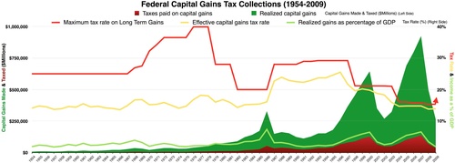
.gif)


.gif)


