Statistical model

From Wikipedia, the free encyclopedia

https://en.wikipedia.org/wiki/Statistical_model

A statistical model is a mathematical model that embodies a set of statistical assumptions concerning the generation of sample data (and similar data from a larger population). A statistical model represents, often in considerably idealized form, the data-generating process. When referring specifically to probabilities, the corresponding term is probabilistic model.

A statistical model is usually specified as a mathematical relationship between one or more random variables and other non-random variables. As such, a statistical model is "a formal representation of a theory" (Herman Adèr quoting Kenneth Bollen).

All statistical hypothesis tests and all statistical estimators are derived via statistical models. More generally, statistical models are part of the foundation of statistical inference.

Introduction

Informally, a statistical model can be thought of as a statistical assumption (or set of statistical assumptions) with a certain property: that the assumption allows us to calculate the probability of any event. As an example, consider a pair of ordinary six-sided dice. We will study two different statistical assumptions about the dice.

The first statistical assumption is this: for each of the dice, the probability of each face (1, 2, 3, 4, 5, and 6) coming up is 1/6. From that assumption, we can calculate the probability of both dice coming up 5:  1/6 × 1/6 = 1/36.  More generally, we can calculate the probability of any event: e.g. (1 and 2) or (3 and 3) or (5 and 6).

The alternative statistical assumption is this: for each of the dice, the probability of the face 5 coming up is 1/8 (because the dice are weighted). From that assumption, we can calculate the probability of both dice coming up 5:  1/8 × 1/8 = 1/64.  We cannot, however, calculate the probability of any other nontrivial event, as the probabilities of the other faces are unknown.

The first statistical assumption constitutes a statistical model: because with the assumption alone, we can calculate the probability of any event. The alternative statistical assumption does not constitute a statistical model: because with the assumption alone, we cannot calculate the probability of every event.

In the example above, with the first assumption, calculating the probability of an event is easy. With some other examples, though, the calculation can be difficult, or even impractical (e.g. it might require millions of years of computation). For an assumption to constitute a statistical model, such difficulty is acceptable: doing the calculation does not need to be practicable, just theoretically possible.

Formal definition

In mathematical terms, a statistical model is usually thought of as a pair (${\displaystyle S,\mathcal{P}}$), where ${\displaystyle S}$ is the set of possible observations, i.e. the sample space, and ${\displaystyle \mathcal{P}}$ is a set of probability distributions on ${\displaystyle S}$.

The intuition behind this definition is as follows. It is assumed that there is a "true" probability distribution induced by the process that generates the observed data. We choose ${\displaystyle \mathcal{P}}$ to represent a set (of distributions) which contains a distribution that adequately approximates the true distribution.

Note that we do not require that ${\displaystyle \mathcal{P}}$ contains the true distribution, and in practice that is rarely the case. Indeed, as Burnham & Anderson state, "A model is a simplification or approximation of reality and hence will not reflect all of reality"—hence the saying "all models are wrong".

The set ${\displaystyle \mathcal{P}}$ is almost always parameterized: ${\displaystyle \mathcal{P}=\{F_{\theta }:\theta \in \mathrm{\Theta }\}}$. The set of distributions ${\displaystyle \mathrm{\Theta }}$ defines the parameters of the model. A parameterization is generally required to have distinct parameter values give rise to distinct distributions, i.e. ${\displaystyle F_{{\theta }_1}=F_{{\theta }_2}\Rightarrow {\theta }_1={\theta }_2}$ must hold (in other words, it must be injective). A parameterization that meets the requirement is said to be identifiable.

An example

Suppose that we have a population of children, with the ages of the children distributed uniformly, in the population. The height of a child will be stochastically related to the age: e.g. when we know that a child is of age 7, this influences the chance of the child being 1.5 meters tall. We could formalize that relationship in a linear regression model, like this: height_i = b₀ + b₁age_i + ε_i, where b₀ is the intercept, b₁ is a parameter that age is multiplied by to obtain a prediction of height, ε_i is the error term, and i identifies the child. This implies that height is predicted by age, with some error.

An admissible model must be consistent with all the data points. Thus, a straight line (height_i = b₀ + b₁age_i) cannot be the equation for a model of the data—unless it exactly fits all the data points, i.e. all the data points lie perfectly on the line. The error term, ε_i, must be included in the equation, so that the model is consistent with all the data points.

To do statistical inference, we would first need to assume some probability distributions for the ε_i. For instance, we might assume that the ε_i distributions are i.i.d. Gaussian, with zero mean. In this instance, the model would have 3 parameters: b₀, b₁, and the variance of the Gaussian distribution.

We can formally specify the model in the form (${\displaystyle S,\mathcal{P}}$) as follows. The sample space, ${\displaystyle S}$, of our model comprises the set of all possible pairs (age, height). Each possible value of ${\displaystyle \theta }$ = (b₀, b₁, σ²) determines a distribution on ${\displaystyle S}$; denote that distribution by ${\displaystyle F_{\theta }}$. If ${\displaystyle \mathrm{\Theta }}$ is the set of all possible values of ${\displaystyle \theta }$, then ${\displaystyle \mathcal{P}=\{F_{\theta }:\theta \in \mathrm{\Theta }\}}$. (The parameterization is identifiable, and this is easy to check.)

In this example, the model is determined by (1) specifying ${\displaystyle S}$ and (2) making some assumptions relevant to ${\displaystyle \mathcal{P}}$. There are two assumptions: that height can be approximated by a linear function of age; that errors in the approximation are distributed as i.i.d. Gaussian. The assumptions are sufficient to specify ${\displaystyle \mathcal{P}}$—as they are required to do.

General remarks

A statistical model is a special class of mathematical model. What distinguishes a statistical model from other mathematical models is that a statistical model is non-deterministic. Thus, in a statistical model specified via mathematical equations, some of the variables do not have specific values, but instead have probability distributions; i.e. some of the variables are stochastic. In the above example with children's heights, ε is a stochastic variable; without that stochastic variable, the model would be deterministic.

Statistical models are often used even when the data-generating process being modeled is deterministic. For instance, coin tossing is, in principle, a deterministic process; yet it is commonly modeled as stochastic (via a Bernoulli process).

Choosing an appropriate statistical model to represent a given data-generating process is sometimes extremely difficult, and may require knowledge of both the process and relevant statistical analyses. Relatedly, the statistician Sir David Cox has said, "How [the] translation from subject-matter problem to statistical model is done is often the most critical part of an analysis".

There are three purposes for a statistical model, according to Konishi & Kitagawa.

• Predictions
• Extraction of information
• Description of stochastic structures

Those three purposes are essentially the same as the three purposes indicated by Friendly & Meyer: prediction, estimation, description. The three purposes correspond with the three kinds of logical reasoning: deductive reasoning, inductive reasoning, abductive reasoning.

Dimension of a model

Suppose that we have a statistical model (${\displaystyle S,\mathcal{P}}$) with ${\displaystyle \mathcal{P}=\{F_{\theta }:\theta \in \mathrm{\Theta }\}}$. In notation, we write that ${\displaystyle \mathrm{\Theta }\subseteq {\mathbb{R}}^k}$ where k is a positive integer (${\displaystyle \mathbb{R}}$ denotes the real numbers; other sets can be used, in principle). Here, k is called the dimension of the model. The model is said to be parametric if ${\displaystyle \mathrm{\Theta }}$ has finite dimension.

As an example, if we assume that data arise from a univariate Gaussian distribution, then we are assuming that

${\displaystyle \mathcal{P}=\left\{F_{\mu ,\sigma }(x)\equiv \frac{1}{\sqrt{2\pi }\sigma }\exp \left(-\frac{(x-\mu {)}^2}{2{\sigma }^2}\right):\mu \in \mathbb{R},\sigma >0\right\}}$.

In this example, the dimension, k, equals 2.

As another example, suppose that the data consists of points (x, y) that we assume are distributed according to a straight line with i.i.d. Gaussian residuals (with zero mean): this leads to the same statistical model as was used in the example with children's heights. The dimension of the statistical model is 3: the intercept of the line, the slope of the line, and the variance of the distribution of the residuals. (Note the set of all possible lines has dimension 2, even though geometrically, a line has dimension 1.)

Although formally ${\displaystyle \theta \in \mathrm{\Theta }}$ is a single parameter that has dimension k, it is sometimes regarded as comprising k separate parameters. For example, with the univariate Gaussian distribution, ${\displaystyle \theta }$ is formally a single parameter with dimension 2, but it is often regarded as comprising 2 separate parameters—the mean and the standard deviation.

A statistical model is nonparametric if the parameter set ${\displaystyle \mathrm{\Theta }}$ is infinite dimensional. A statistical model is semiparametric if it has both finite-dimensional and infinite-dimensional parameters. Formally, if k is the dimension of ${\displaystyle \mathrm{\Theta }}$ and n is the number of samples, both semiparametric and nonparametric models have ${\displaystyle k\to \mathrm{\infty }}$ as ${\displaystyle n\to \mathrm{\infty }}$. If ${\displaystyle k/n\to 0}$ as ${\displaystyle n\to \mathrm{\infty }}$, then the model is semiparametric; otherwise, the model is nonparametric.

Parametric models are by far the most commonly used statistical models. Regarding semiparametric and nonparametric models, Sir David Cox has said, "These typically involve fewer assumptions of structure and distributional form but usually contain strong assumptions about independencies".

Nested models

Not to be confused with Multilevel models.

Two statistical models are nested if the first model can be transformed into the second model by imposing constraints on the parameters of the first model. As an example, the set of all Gaussian distributions has, nested within it, the set of zero-mean Gaussian distributions: we constrain the mean in the set of all Gaussian distributions to get the zero-mean distributions. As a second example, the quadratic model

y = b₀ + b₁x + b₂x² + ε,    ε ~ 𝒩(0, σ²)

has, nested within it, the linear model

y = b₀ + b₁x + ε,    ε ~ 𝒩(0, σ²)

—we constrain the parameter b₂ to equal 0.

In both those examples, the first model has a higher dimension than the second model (for the first example, the zero-mean model has dimension 1). Such is often, but not always, the case. As a example where they have the same dimension, the set of positive-mean Gaussian distributions is nested within the set of all Gaussian distributions; they both have dimension 2.

Comparing models

See also: Statistical model selection

Comparing statistical models is fundamental for much of statistical inference. Indeed, Konishi & Kitagawa (2008, p. 75) state this: "The majority of the problems in statistical inference can be considered to be problems related to statistical modeling. They are typically formulated as comparisons of several statistical models."

Common criteria for comparing models include the following: R², Bayes factor, Akaike information criterion, and the likelihood-ratio test together with its generalization, the relative likelihood.

Volatile organic compound

From Wikipedia, the free encyclopedia

https://en.wikipedia.org/wiki/Volatile_organic_compound

Volatile organic compounds (VOCs) are organic compounds that have a high vapor pressure at room temperature. High vapor pressure correlates with a low boiling point, which relates to the number of the sample's molecules in the surrounding air, a trait known as volatility.

VOCs are responsible for the odor of scents and perfumes as well as pollutants. VOCs play an important role in communication between animals and plants, e.g. attractants for pollinators, protection from predation, and even inter-plant interactions. Some VOCs are dangerous to human health or cause harm to the environment. Anthropogenic VOCs are regulated by law, especially indoors, where concentrations are the highest. Most VOCs are not acutely toxic, but may have long-term chronic health effects. Some VOCs have been used in pharmacy, while others are target of administrative controls because of their recreational use.

Definitions

Diverse definitions of the term VOC are in use. Some examples are presented below.

Canada

Health Canada classifies VOCs as organic compounds that have boiling points roughly in the range of 50 to 250 °C (122 to 482 °F). The emphasis is placed on commonly encountered VOCs that would have an effect on air quality.

European Union

The European Union defines a VOC as "any organic compound as well as the fraction of creosote, having at 293.15 K a vapour pressure of 0,01 kPa or more, or having a corresponding volatility under the particular conditions of use". The VOC Solvents Emissions Directive was the main policy instrument for the reduction of industrial emissions of volatile organic compounds (VOCs) in the European Union. It covers a wide range of solvent-using activities, e.g. printing, surface cleaning, vehicle coating, dry cleaning and manufacture of footwear and pharmaceutical products. The VOC Solvents Emissions Directive requires installations in which such activities are applied to comply either with the emission limit values set out in the Directive or with the requirements of the so-called reduction scheme. Article 13 of The Paints Directive, approved in 2004, amended the original VOC Solvents Emissions Directive and limits the use of organic solvents in decorative paints and varnishes and in vehicle finishing products. The Paints Directive sets out maximum VOC content limit values for paints and varnishes in certain applications. The Solvents Emissions Directive was replaced by the Industrial Emissions Directive from 2013.

China

The People's Republic of China defines a VOC as those compounds that have "originated from automobiles, industrial production and civilian use, burning of all types of fuels, storage and transportation of oils, fitment finish, coating for furniture and machines, cooking oil fume and fine particles (PM 2.5)", and similar sources. The Three-Year Action Plan for Winning the Blue Sky Defence War released by the State Council in July 2018 creates an action plan to reduce 2015 VOC emissions 10% by 2020.

India

The Central Pollution Control Board of India released the Air (Prevention and Control of Pollution) Act in 1981, amended in 1987, to address concerns about air pollution in India. While the document does not differentiate between VOCs and other air pollutants, the CPCB monitors "oxides of nitrogen (NO_x), sulphur dioxide (SO₂), fine particulate matter (PM10) and suspended particulate matter (SPM)".

United States

Thermal oxidizers provide an air pollution abatement option for VOCs from industrial air flows. A thermal oxidizer is an EPA-approved device to treat VOCs.

The definitions of VOCs used for control of precursors of photochemical smog used by the U.S. Environmental Protection Agency (EPA) and state agencies in the US with independent outdoor air pollution regulations include exemptions for VOCs that are determined to be non-reactive, or of low-reactivity in the smog formation process. Prominent is the VOC regulation issued by the South Coast Air Quality Management District in California and by the California Air Resources Board (CARB). However, this specific use of the term VOCs can be misleading, especially when applied to indoor air quality because many chemicals that are not regulated as outdoor air pollution can still be important for indoor air pollution.

Following a public hearing in September 1995, California's ARB uses the term "reactive organic gases" (ROG) to measure organic gases. The CARB revised the definition of "Volatile Organic Compounds" used in their consumer products regulations, based on the committee's findings.

In addition to drinking water, VOCs are regulated in pollutant discharges to surface waters (both directly and via sewage treatment plants) as hazardous waste, but not in non-industrial indoor air. The Occupational Safety and Health Administration (OSHA) regulates VOC exposure in the workplace. Volatile organic compounds that are classified as hazardous materials are regulated by the Pipeline and Hazardous Materials Safety Administration while being transported.

Biologically generated VOCs

• 

  Limonene, a common biogenic VOC, is emitted into the atmosphere primarily by trees which grow in coniferous forests.

Most VOCs in Earth's atmosphere are biogenic, largely emitted by plants.

Major biogenic VOCs

compound	relative contribution	amount emitted (Tg/y)
isoprene	62.2%	594±34
terpenes	10.9%	95±3
pinene isomers	5.6%	48.7±0.8
sesquiterpenes	2.4%	20±1
methanol	6.4%	130±4

Biogenic volatile organic compounds (BVOCs) encompass VOCs emitted by plants, animals, or microorganisms, and while extremely diverse, are most commonly terpenoids, alcohols, and carbonyls (methane and carbon monoxide are generally not considered). Not counting methane, biological sources emit an estimated 760 teragrams of carbon per year in the form of VOCs. The majority of VOCs are produced by plants, the main compound being isoprene. Small amounts of VOCs are produced by animals and microbes. Many VOCs are considered secondary metabolites, which often help organisms in defense, such as plant defense against herbivory. The strong odor emitted by many plants consists of green leaf volatiles, a subset of VOCs. Although intended for nearby organisms to detect and respond to, these volatiles can be detected and communicated through wireless electronic transmission, by embedding nanosensors and infrared transmitters into the plant materials themselves.

Emissions are affected by a variety of factors, such as temperature, which determines rates of volatilization and growth, and sunlight, which determines rates of biosynthesis. Emission occurs almost exclusively from the leaves, the stomata in particular. VOCs emitted by terrestrial forests are often oxidized by hydroxyl radicals in the atmosphere; in the absence of NO_x pollutants, VOC photochemistry recycles hydroxyl radicals to create a sustainable biosphere-atmosphere balance. Due to recent climate change developments, such as warming and greater UV radiation, BVOC emissions from plants are generally predicted to increase, thus upsetting the biosphere-atmosphere interaction and damaging major ecosystems. A major class of VOCs is the terpene class of compounds, such as myrcene.

Providing a sense of scale, a forest 62,000 square kilometres (24,000 sq mi) in area, the size of the US state of Pennsylvania, is estimated to emit 3,400,000 kilograms (7,500,000 lb) of terpenes on a typical August day during the growing season. Researchers investigating mechanisms of induction of genes producing volatile organic compounds, and the subsequent increase in volatile terpenes, has been achieved in maize using (Z)-3-hexen-1-ol and other plant hormones.

Anthropogenic sources

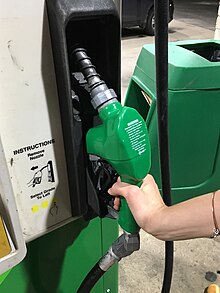
The handling of petroleum-based fuels is a major source of VOCs.

Anthropogenic sources emit about 142 teragrams (1.42 × 10¹¹ kg) of carbon per year in the form of VOCs.

The major source of man-made VOCs are:

• Fossil fuel use and production, e.g. incompletely combusted fossil fuels or unintended evaporation of fuels. The most prevalent VOC is ethane, a relatively inert compound.
• Solvents used in coatings, paints, and inks. Approximately 12 billion litres of paint are produced annually. Typical solvents include aliphatic hydrocarbons, ethyl acetate, glycol ethers, and acetone. Motivated by cost, environmental concerns, and regulation, the paint and coating industries are increasingly shifting toward aqueous solvents.
• Compressed aerosol products, mainly butane and propane, estimated to contribute 1.3 billion tonnes of VOC emissions per year globally.
• Biofuel use, e.g., cooking oils in Asia and bioethanol in Brazil.
• Biomass combustion, especially from rain forests. Although combustion principally releases carbon dioxide and water, incomplete combustion affords a variety of VOCs.

Indoor VOCs

Concentrations of VOCs in indoor air may be 2 to 5 times greater than in outdoor air, sometimes far greater. During certain activities, indoor levels of VOCs may reach 1,000 times that of the outside air. Studies have shown that emissions of individual VOC species are not that high in an indoor environment, but the total concentration of all VOCs (TVOC) indoors can be up to five times higher than that of outdoor levels.

New buildings experience particularly high levels of VOC off-gassing indoors because of the abundant new materials (building materials, fittings, surface coverings and treatments such as glues, paints and sealants) exposed to the indoor air, emitting multiple VOC gases. This off-gassing has a multi-exponential decay trend that is discernible over at least two years, with the most volatile compounds decaying with a time-constant of a few days, and the least volatile compounds decaying with a time-constant of a few years.

New buildings may require intensive ventilation for the first few months, or a bake-out treatment. Existing buildings may be replenished with new VOC sources, such as new furniture, consumer products, and redecoration of indoor surfaces, all of which lead to a continuous background emission of TVOCs, and requiring improved ventilation.

Numerous studies show strong seasonal variations in indoors VOC emissions, with emission rates increasing in summer. This is largely due to the rate of diffusion of VOC species through materials to the surface, increasing with temperature. Most studies have shown that this leads to generally higher concentrations of TVOCs indoors in summer.

Indoor air quality measurements

Measurement of VOCs from the indoor air is done with sorption tubes e. g. Tenax (for VOCs and SVOCs) or DNPH-cartridges (for carbonyl-compounds) or air detector. The VOCs adsorb on these materials and are afterwards desorbed either thermally (Tenax) or by elution (DNPH) and then analyzed by GC-MS/FID or HPLC. Reference gas mixtures are required for quality control of these VOC-measurements. Furthermore, VOC emitting products used indoors, e.g. building products and furniture, are investigated in emission test chambers under controlled climatic conditions. For quality control of these measurements round robin tests are carried out, therefore reproducibly emitting reference materials are ideally required. Other methods have used proprietary Silcosteel-coated canisters with constant flow inlets to collect samples over several days. These methods are not limited by the adsorbing properties of materials like Tenax.

Regulation of indoor VOC emissions

In most countries, a separate definition of VOCs is used with regard to indoor air quality that comprises each organic chemical compound that can be measured as follows: adsorption from air on Tenax TA, thermal desorption, gas chromatographic separation over a 100% nonpolar column (dimethylpolysiloxane). VOC (volatile organic compounds) are all compounds that appear in the gas chromatogram between and including n-hexane and n-hexadecane. Compounds appearing earlier are called VVOC (very volatile organic compounds); compounds appearing later are called SVOC (semi-volatile organic compounds).

France, Germany (AgBB/DIBt), Belgium, Norway (TEK regulation), and Italy (CAM Edilizia) have enacted regulations to limit VOC emissions from commercial products. European industry has developed numerous voluntary ecolabels and rating systems, such as EMICODE, M1, Blue Angel, GuT (textile floor coverings), Nordic Swan Ecolabel, EU Ecolabel, and Indoor Air Comfort. In the United States, several standards exist; California Standard CDPH Section 01350 is the most common one. These regulations and standards changed the marketplace, leading to an increasing number of low-emitting products.

Health risks

See also: Chronic solvent-induced encephalopathy and Substance-induced psychosis

Respiratory, allergic, or immune effects in infants or children are associated with man-made VOCs and other indoor or outdoor air pollutants.

Some VOCs, such as styrene and limonene, can react with nitrogen oxides or with ozone to produce new oxidation products and secondary aerosols, which can cause sensory irritation symptoms. VOCs contribute to the formation of tropospheric ozone and smog.

Health effects include eye, nose, and throat irritation; headaches, loss of coordination, nausea; and damage to the liver, kidney, and central nervous system. Some organics can cause cancer in animals; some are suspected or known to cause cancer in humans. Key signs or symptoms associated with exposure to VOCs include conjunctival irritation, nose and throat discomfort, headache, allergic skin reaction, dyspnea, declines in serum cholinesterase levels, nausea, vomiting, nose bleeding, fatigue, dizziness.

The ability of organic chemicals to cause health effects varies greatly from those that are highly toxic to those with no known health effects. As with other pollutants, the extent and nature of the health effect will depend on many factors including level of exposure and length of time exposed. Eye and respiratory tract irritation, headaches, dizziness, visual disorders, and memory impairment are among the immediate symptoms that some people have experienced soon after exposure to some organics. At present, not much is known about what health effects occur from the levels of organics usually found in homes.

Ingestion

While null in comparison to the concentrations found in indoor air, benzene, toluene, and methyl tert-butyl ether (MTBE) were found in samples of human milk and increase the concentrations of VOCs that we are exposed to throughout the day. A study notes the difference between VOCs in alveolar breath and inspired air suggesting that VOCs are ingested, metabolized, and excreted via the extra-pulmonary pathway. VOCs are also ingested by drinking water in varying concentrations. Some VOC concentrations were over the EPA’s National Primary Drinking Water Regulations and China’s National Drinking Water Standards set by the Ministry of Ecology and Environment.

Dermal absorption

The presence of VOCs in the air and in groundwater has prompted more studies. Several studies have been performed to measure the effects of dermal absorption of specific VOCs. Dermal exposure to VOCs like formaldehyde and toluene downregulate antimicrobial peptides on the skin like cathelicidin LL-37, human β-defensin 2 and 3. Xylene and formaldehyde worsen allergic inflammation in animal models. Toluene also increases the dysregulation of filaggrin: a key protein in dermal regulation. this was confirmed by immunofluorescence to confirm protein loss and western blotting to confirm mRNA loss. These experiments were done on human skin samples. Toluene exposure also decreased the water in the trans-epidermal layer allowing for vulnerability in the skin’s layers.

Limit values for VOC emissions

Limit values for VOC emissions into indoor air are published by AgBB, AFSSET, California Department of Public Health, and others. These regulations have prompted several companies in the paint and adhesive industries to adapt with VOC level reductions their products. VOC labels and certification programs may not properly assess all of the VOCs emitted from the product, including some chemical compounds that may be relevant for indoor air quality. Each ounce of colorant added to tint paint may contain between 5 and 20 grams of VOCs. A dark color, however, could require 5–15 ounces of colorant, adding up to 300 or more grams of VOCs per gallon of paint.

VOCs in healthcare settings

VOCs are also found in hospital and health care environments. In these settings, these chemicals are widely used for cleaning, disinfection, and hygiene of the different areas. Thus, health professionals such as nurses, doctors, sanitation staff, etc., may present with adverse health effects such as asthma; however, further evaluation is required to determine the exact levels and determinants that influence the exposure to these compounds.

Studies have shown that the concentration levels of different VOCs such as halogenated and aromatic hydrocarbons differ substantially between areas of the same hospital. However, one of these studies reported that ethanol, isopropanol, ether, and acetone were the main compounds in the interior of the site. Following the same line, in a study conducted in the United States, it was established that nursing assistants are the most exposed to compounds such as ethanol, while medical equipment preparers are most exposed to 2-propanol.

In relation to exposure to VOCs by cleaning and hygiene personnel, a study conducted in 4 hospitals in the United States established that sterilization and disinfection workers are linked to exposures to d-limonene and 2-propanol, while those responsible for cleaning with chlorine-containing products are more likely to have higher levels of exposure to α-pinene and chloroform. Those who perform floor and other surface cleaning tasks (e.g., floor waxing) and who use quaternary ammonium, alcohol, and chlorine-based products are associated with a higher VOC exposure than the two previous groups, that is, they are particularly linked to exposure to acetone, chloroform, α-pinene, 2-propanol or d-limonene.

Other healthcare environments such as nursing and age care homes have been rarely a subject of study, even though the elderly and vulnerable populations may spend considerable time in these indoor settings where they might be exposed to VOCs, derived from the common use of cleaning agents, sprays and fresheners. In a study conducted in France, a team of researchers developed an online questionnaire for different social and age care facilities, asking about cleaning practices, products used, and the frequency of these activities. As a result, more than 200 chemicals were identified, of which 41 are known to have adverse health effects, 37 of them being VOCs. The health effects include skin sensitization, reproductive and organ-specific toxicity, carcinogenicity, mutagenicity, and endocrine-disrupting properties. Furthermore, in another study carried out in the same European country, it was found that there is a significant association between breathlessness in the elderly population and elevated exposure to VOCs such as toluene and o-xylene, unlike the remainder of the population.

Analytical methods

Sampling

Obtaining samples for analysis is challenging. VOCs, even when at dangerous levels, are dilute, so preconcentration is typically required. Many components of the atmosphere are mutually incompatible, e.g. ozone and organic compounds, peroxyacyl nitrates and many organic compounds. Furthermore, collection of VOCs by condensation in cold traps also accumulates a large amount of water, which generally must be removed selectively, depending on the analytical techniques to be employed. Solid-phase microextraction (SPME) techniques are used to collect VOCs at low concentrations for analysis. As applied to breath analysis, the following modalities are employed for sampling: gas sampling bags, syringes, evacuated steel and glass containers.

Principle and measurement methods

In the U.S., standard methods have been established by the National Institute for Occupational Safety and Health (NIOSH) and another by U.S. OSHA. Each method uses a single component solvent; butanol and hexane cannot be sampled, however, on the same sample matrix using the NIOSH or OSHA method.

VOCs are quantified and identified by two broad techniques. The major technique is gas chromatography (GC). GC instruments allow the separation of gaseous components. When coupled to a flame ionization detector (FID) GCs can detect hydrocarbons at the parts per trillion levels. Using electron capture detectors, GCs are also effective for organohalide such as chlorocarbons.

The second major technique associated with VOC analysis is mass spectrometry, which is usually coupled with GC, giving the hyphenated technique of GC-MS.

Direct injection mass spectrometry techniques are frequently utilized for the rapid detection and accurate quantification of VOCs. PTR-MS is among the methods that have been used most extensively for the on-line analysis of biogenic and anthropogenic VOCs. PTR-MS instruments based on time-of-flight mass spectrometry have been reported to reach detection limits of 20 pptv after 100 ms and 750 ppqv after 1 min. measurement (signal integration) time. The mass resolution of these devices is between 7000 and 10,500 m/Δm, thus it is possible to separate most common isobaric VOCs and quantify them independently.

Chemical fingerprinting and breath analysis

The exhaled human breath contains a few thousand volatile organic compounds and is used in breath biopsy to serve as a VOC biomarker to test for diseases, such as lung cancer. One study has shown that "volatile organic compounds ... are mainly blood borne and therefore enable monitoring of different processes in the body." And it appears that VOC compounds in the body "may be either produced by metabolic processes or inhaled/absorbed from exogenous sources" such as environmental tobacco smoke. Chemical fingerprinting and breath analysis of volatile organic compounds has also been demonstrated with chemical sensor arrays, which utilize pattern recognition for detection of component volatile organics in complex mixtures such as breath gas.

Metrology for VOC measurements

To achieve comparability of VOC measurements, reference standards traceable to SI-units are required. For a number of VOCs gaseous reference standards are available from specialty gas suppliers or national metrology institutes, either in the form of cylinders or dynamic generation methods. However, for many VOCs, such as oxygenated VOCs, monoterpenes, or formaldehyde, no standards are available at the appropriate amount of fraction due to the chemical reactivity or adsorption of these molecules. Currently, several national metrology institutes are working on the lacking standard gas mixtures at trace level concentration, minimising adsorption processes, and improving the zero gas. The final scopes are for the traceability and the long-term stability of the standard gases to be in accordance with the data quality objectives (DQO, maximum uncertainty of 20% in this case) required by the WMO/GAW program.

Gaussian process

From Wikipedia, the free encyclopedia

https://en.wikipedia.org/wiki/Gaussian_process 

In probability theory and statistics, a Gaussian process is a stochastic process (a collection of random variables indexed by time or space), such that every finite collection of those random variables has a multivariate normal distribution, i.e. every finite linear combination of them is normally distributed. The distribution of a Gaussian process is the joint distribution of all those (infinitely many) random variables, and as such, it is a distribution over functions with a continuous domain, e.g. time or space.

The concept of Gaussian processes is named after Carl Friedrich Gauss because it is based on the notion of the Gaussian distribution (normal distribution). Gaussian processes can be seen as an infinite-dimensional generalization of multivariate normal distributions.

Gaussian processes are useful in statistical modelling, benefiting from properties inherited from the normal distribution. For example, if a random process is modelled as a Gaussian process, the distributions of various derived quantities can be obtained explicitly. Such quantities include the average value of the process over a range of times and the error in estimating the average using sample values at a small set of times. While exact models often scale poorly as the amount of data increases, multiple approximation methods have been developed which often retain good accuracy while drastically reducing computation time.

Definition

A time continuous stochastic process ${\displaystyle \left\{X_t;t\in T\right\}}$ is Gaussian if and only if for every finite set of indices ${\displaystyle t_1,\dots ,t_k}$ in the index set ${\displaystyle T}$

$${\displaystyle {\mathbf{X}}_{t_1,\dots ,t_k}=(X_{t_1},\dots ,X_{t_k})}$$

is a multivariate Gaussian random variable. That is the same as saying every linear combination of ${\displaystyle (X_{t_1},\dots ,X_{t_k})}$ has a univariate normal (or Gaussian) distribution.

Using characteristic functions of random variables, the Gaussian property can be formulated as follows: ${\displaystyle \left\{X_t;t\in T\right\}}$ is Gaussian if and only if, for every finite set of indices ${\displaystyle t_1,\dots ,t_k}$, there are real-valued ${\displaystyle {\sigma }_{\ell j}}$, ${\displaystyle {\mu }_{\ell }}$ with ${\displaystyle {\sigma }_{jj}>0}$ such that the following equality holds for all ${\displaystyle s_1,s_2,\dots ,s_k\in \mathbb{R}}$

$${\displaystyle \mathrm{E}\left(\exp \left(i\sum _{\ell =1}^k{s}_{\ell }{\mathbf{X}}_{t_{\ell }}\right)\right)=\exp \left(-\frac{1}{2}\sum _{\ell ,j}{\sigma }_{\ell j}{s}_{\ell }{s}_j+i\sum _{\ell }{\mu }_{\ell }{s}_{\ell }\right),}$$

where ${\displaystyle i}$ denotes the imaginary unit such that ${\displaystyle i^2=-1}$.

The numbers ${\displaystyle {\sigma }_{\ell j}}$ and ${\displaystyle {\mu }_{\ell }}$ can be shown to be the covariances and means of the variables in the process.

Variance

The variance of a Gaussian process is finite at any time ${\displaystyle t}$, formally

$${\displaystyle \mathrm{var}[X(t)]=\mathrm{E}\left[{\left|X(t)-\mathrm{E}[X(t)]\right|}^2\right]<\mathrm{\infty }\text{for all }t\in T.}$$

Stationarity

For general stochastic processes strict-sense stationarity implies wide-sense stationarity but not every wide-sense stationary stochastic process is strict-sense stationary. However, for a Gaussian stochastic process the two concepts are equivalent.

A Gaussian stochastic process is strict-sense stationary if, and only if, it is wide-sense stationary.

Example

There is an explicit representation for stationary Gaussian processes. A simple example of this representation is

$${\displaystyle X_t=\cos (at){\xi }_1+\sin (at){\xi }_2}$$

where ${\displaystyle {\xi }_1}$ and ${\displaystyle {\xi }_2}$ are independent random variables with the standard normal distribution.

Covariance functions

Main article: Covariance function

Further information: Variogram

A key fact of Gaussian processes is that they can be completely defined by their second-order statistics. Thus, if a Gaussian process is assumed to have mean zero, defining the covariance function completely defines the process' behaviour. Importantly the non-negative definiteness of this function enables its spectral decomposition using the Karhunen–Loève expansion. Basic aspects that can be defined through the covariance function are the process' stationarity, isotropy, smoothness and periodicity.

Stationarity refers to the process' behaviour regarding the separation of any two points ${\displaystyle x}$ and ${\displaystyle x^{\prime }}$. If the process is stationary, the covariance function depends only on ${\displaystyle x-x^{\prime }}$. For example, the Ornstein–Uhlenbeck process is stationary.

If the process depends only on ${\displaystyle |x-x^{\prime }|}$, the Euclidean distance (not the direction) between ${\displaystyle x}$ and ${\displaystyle x^{\prime }}$, then the process is considered isotropic. A process that is concurrently stationary and isotropic is considered to be homogeneous; in practice these properties reflect the differences (or rather the lack of them) in the behaviour of the process given the location of the observer.

Ultimately Gaussian processes translate as taking priors on functions and the smoothness of these priors can be induced by the covariance function. If we expect that for "near-by" input points ${\displaystyle x}$ and ${\displaystyle x^{\prime }}$ their corresponding output points ${\displaystyle y}$ and ${\displaystyle y^{\prime }}$ to be "near-by" also, then the assumption of continuity is present. If we wish to allow for significant displacement then we might choose a rougher covariance function. Extreme examples of the behaviour is the Ornstein–Uhlenbeck covariance function and the squared exponential where the former is never differentiable and the latter infinitely differentiable.

Periodicity refers to inducing periodic patterns within the behaviour of the process. Formally, this is achieved by mapping the input ${\displaystyle x}$ to a two dimensional vector ${\displaystyle u(x)=\left(\cos (x),\sin (x)\right)}$.

Usual covariance functions

The effect of choosing different kernels on the prior function distribution of the Gaussian process. Left is a squared exponential kernel. Middle is Brownian. Right is quadratic.

There are a number of common covariance functions:

• Constant : ${\displaystyle K_{\mathrm{C}}(x,x^{\prime })=C}$
• Linear: ${\displaystyle K_{\mathrm{L}}(x,x^{\prime })=x^{\mathsf{T}}{x}^{\prime }}$
• white Gaussian noise: ${\displaystyle K_{\mathrm{GN}}(x,x^{\prime })={\sigma }^2{\delta }_{x,x^{\prime }}}$
• Squared exponential: ${\displaystyle K_{\mathrm{SE}}(x,x^{\prime })=\exp \left(-\frac{|d{|}^2}{2{\ell }^2}\right)}$
• Ornstein–Uhlenbeck: ${\displaystyle K_{\mathrm{OU}}(x,x^{\prime })=\exp \left(-\frac{|d|}{\ell }\right)}$
• Matérn: ${\displaystyle K_{\mathrm{Matern}}(x,x^{\prime })=\frac{2^{1-\nu }}{\mathrm{\Gamma }(\nu )}{\left(\frac{\sqrt{2\nu }|d|}{\ell }\right)}^{\nu }{K}_{\nu }\left(\frac{\sqrt{2\nu }|d|}{\ell }\right)}$
• Periodic: ${\displaystyle K_{\mathrm{P}}(x,x^{\prime })=\exp \left(-\frac{2{\sin }^2\left(\frac{d}{2}\right)}{{\ell }^2}\right)}$
• Rational quadratic: ${\displaystyle K_{\mathrm{RQ}}(x,x^{\prime })={\left(1+|d{|}^2\right)}^{-\alpha },\alpha \ge 0}$

Here ${\displaystyle d=x-x^{\prime }}$. The parameter ${\displaystyle \ell }$ is the characteristic length-scale of the process (practically, "how close" two points ${\displaystyle x}$ and ${\displaystyle x^{\prime }}$ have to be to influence each other significantly), ${\displaystyle \delta }$ is the Kronecker delta and ${\displaystyle \sigma }$ the standard deviation of the noise fluctuations. Moreover, ${\displaystyle K_{\nu }}$ is the modified Bessel function of order ${\displaystyle \nu }$ and ${\displaystyle \mathrm{\Gamma }(\nu )}$ is the gamma function evaluated at ${\displaystyle \nu }$. Importantly, a complicated covariance function can be defined as a linear combination of other simpler covariance functions in order to incorporate different insights about the data-set at hand.

The inferential results are dependent on the values of the hyperparameters ${\displaystyle \theta }$ (e.g. ${\displaystyle \ell }$ and ${\displaystyle \sigma }$) defining the model's behaviour. A popular choice for ${\displaystyle \theta }$ is to provide maximum a posteriori (MAP) estimates of it with some chosen prior. If the prior is very near uniform, this is the same as maximizing the marginal likelihood of the process; the marginalization being done over the observed process values ${\displaystyle y}$. This approach is also known as maximum likelihood II, evidence maximization, or empirical Bayes.

Continuity

For a Gaussian process, continuity in probability is equivalent to mean-square continuity, and continuity with probability one is equivalent to sample continuity. The latter implies, but is not implied by, continuity in probability. Continuity in probability holds if and only if the mean and autocovariance are continuous functions. In contrast, sample continuity was challenging even for stationary Gaussian processes (as probably noted first by Andrey Kolmogorov), and more challenging for more general processes. As usual, by a sample continuous process one means a process that admits a sample continuous modification. 

Stationary case

For a stationary Gaussian process ${\displaystyle X=(X_t{)}_{t\in \mathbb{R}},}$ some conditions on its spectrum are sufficient for sample continuity, but fail to be necessary. A necessary and sufficient condition, sometimes called Dudley–Fernique theorem, involves the function ${\displaystyle \sigma }$ defined by

$${\displaystyle \sigma (h)=\sqrt{\mathbb{E}(X(t+h)-X(t){)}^2}}$$

(the right-hand side does not depend on ${\displaystyle t}$ due to stationarity). Continuity of ${\displaystyle X}$ in probability is equivalent to continuity of ${\displaystyle \sigma }$ at ${\displaystyle 0.}$ When convergence of ${\displaystyle \sigma (h)}$ to ${\displaystyle 0}$ (as ${\displaystyle h\to 0}$) is too slow, sample continuity of ${\displaystyle X}$ may fail. Convergence of the following integrals matters:

$${\displaystyle I(\sigma )={\int }_0^1\frac{\sigma (h)}{h\sqrt{\log (1/h)}}dh={\int }_0^{\mathrm{\infty }}2\sigma (e^{-x^2})dx,}$$

these two integrals being equal according to integration by substitution $h=e^{-x^2},$ $x=\sqrt{\log (1/h)}.$ The first integrand need not be bounded as ${\displaystyle h\to 0+,}$ thus the integral may converge (${\displaystyle I(\sigma )<\mathrm{\infty }}$) or diverge (${\displaystyle I(\sigma )=\mathrm{\infty }}$). Taking for example $\sigma (e^{-x^2})=\frac{1}{x^a}$ for large ${\displaystyle x,}$ that is, $\sigma (h)=(\log (1/h){)}^{-a/2}$ for small ${\displaystyle h,}$ one obtains ${\displaystyle I(\sigma )<\mathrm{\infty }}$ when ${\displaystyle a>1,}$ and ${\displaystyle I(\sigma )=\mathrm{\infty }}$ when ${\displaystyle 0<a\le 1.}$ In these two cases the function ${\displaystyle \sigma }$ is increasing on ${\displaystyle [0,\mathrm{\infty }),}$ but generally it is not. Moreover, the condition

(*)   there exists ${\displaystyle \epsilon >0}$ such that ${\displaystyle \sigma }$ is monotone on ${\displaystyle [0,\epsilon ]}$

does not follow from continuity of ${\displaystyle \sigma }$ and the evident relations ${\displaystyle \sigma (h)\ge 0}$ (for all ${\displaystyle h}$) and ${\displaystyle \sigma (0)=0.}$

Theorem 1 — Let ${\displaystyle \sigma }$ be continuous and satisfy (*). Then the condition ${\displaystyle I(\sigma )<\mathrm{\infty }}$ is necessary and sufficient for sample continuity of ${\displaystyle X.}$

Some history. Sufficiency was announced by Xavier Fernique in 1964, but the first proof was published by Richard M. Dudley in 1967. Necessity was proved by Michael B. Marcus and Lawrence Shepp in 1970.

There exist sample continuous processes ${\displaystyle X}$ such that ${\displaystyle I(\sigma )=\mathrm{\infty };}$ they violate condition (*). An example found by Marcus and Shepp  is a random lacunary Fourier series

$${\displaystyle X_t=\sum _{n=1}^{\mathrm{\infty }}{c}_n({\xi }_n\cos {\lambda }_{n}t+{\eta }_n\sin {\lambda }_{n}t),}$$

where ${\displaystyle {\xi }_1,{\eta }_1,{\xi }_2,{\eta }_2,\dots }$ are independent random variables with standard normal distribution; frequencies ${\displaystyle 0<{\lambda }_1<{\lambda }_2<\dots }$ are a fast growing sequence; and coefficients ${\displaystyle c_n>0}$ satisfy $\sum _n{c}_n<\mathrm{\infty }.$ The latter relation implies $\mathbb{E}\sum _n{c}_n(|{\xi }_n|+|{\eta }_n|)=\sum _n{c}_n\mathbb{E}(|{\xi }_n|+|{\eta }_n|)=\text{const}\cdot \sum _n{c}_n<\mathrm{\infty },$ whence $\sum _n{c}_n(|{\xi }_n|+|{\eta }_n|)<\mathrm{\infty }$ almost surely, which ensures uniform convergence of the Fourier series almost surely, and sample continuity of ${\displaystyle X.}$

Autocorrelation of a random lacunary Fourier series

Its autocovariation function

$${\displaystyle \mathbb{E}{X}_t{X}_{t+h}=\sum _{n=1}^{\mathrm{\infty }}{c}_n^2\cos {\lambda }_{n}h}$$

is nowhere monotone (see the picture), as well as the corresponding function ${\displaystyle \sigma ,}$

$${\displaystyle \sigma (h)=\sqrt{2\mathbb{E}{X}_t{X}_t-2\mathbb{E}{X}_t{X}_{t+h}}=2\sqrt{\sum _{n=1}^{\mathrm{\infty }}{c}_n^2{\sin }^2\frac{{\lambda }_{n}h}{2}}.}$$

Brownian motion as the integral of Gaussian processes

A Wiener process (also known as Brownian motion) is the integral of a white noise generalized Gaussian process. It is not stationary, but it has stationary increments.

The Ornstein–Uhlenbeck process is a stationary Gaussian process.

The Brownian bridge is (like the Ornstein–Uhlenbeck process) an example of a Gaussian process whose increments are not independent.

The fractional Brownian motion is a Gaussian process whose covariance function is a generalisation of that of the Wiener process.

Driscoll's zero-one law

Driscoll's zero-one law is a result characterizing the sample functions generated by a Gaussian process.

Let ${\displaystyle f}$ be a mean-zero Gaussian process ${\displaystyle \left\{X_t;t\in T\right\}}$ with non-negative definite covariance function ${\displaystyle K}$. Let ${\displaystyle \mathcal{H}(R)}$ be a Reproducing kernel Hilbert space with positive definite kernel ${\displaystyle R}$.

Then

$${\displaystyle \underset{n\to \mathrm{\infty }}{lim}\mathrm{tr}[K_n{R}_n^{-1}]<\mathrm{\infty },}$$

where ${\displaystyle K_n}$ and ${\displaystyle R_n}$ are the covariance matrices of all possible pairs of ${\displaystyle n}$ points, implies

$${\displaystyle Pr[f\in \mathcal{H}(R)]=1.}$$

Moreover,

$${\displaystyle \underset{n\to \mathrm{\infty }}{lim}\mathrm{tr}[K_n{R}_n^{-1}]=\mathrm{\infty }}$$

implies 

$${\displaystyle Pr[f\in \mathcal{H}(R)]=0.}$$

This has significant implications when ${\displaystyle K=R}$, as

$${\displaystyle \underset{n\to \mathrm{\infty }}{lim}\mathrm{tr}[R_n{R}_n^{-1}]=\underset{n\to \mathrm{\infty }}{lim}\mathrm{tr}[I]=\underset{n\to \mathrm{\infty }}{lim}n=\mathrm{\infty }.}$$

As such, almost all sample paths of a mean-zero Gaussian process with positive definite kernel ${\displaystyle K}$ will lie outside of the Hilbert space ${\displaystyle \mathcal{H}(K)}$.

Linearly constrained Gaussian processes

For many applications of interest some pre-existing knowledge about the system at hand is already given. Consider e.g. the case where the output of the Gaussian process corresponds to a magnetic field; here, the real magnetic field is bound by Maxwell's equations and a way to incorporate this constraint into the Gaussian process formalism would be desirable as this would likely improve the accuracy of the algorithm.

A method on how to incorporate linear constraints into Gaussian processes already exists:

Consider the (vector valued) output function ${\displaystyle f(x)}$ which is known to obey the linear constraint (i.e. ${\displaystyle {\mathcal{F}}_X}$ is a linear operator)

$${\displaystyle {\mathcal{F}}_X(f(x))=0.}$$

Then the constraint ${\displaystyle {\mathcal{F}}_X}$ can be fulfilled by choosing ${\displaystyle f(x)={\mathcal{G}}_X(g(x))}$, where ${\displaystyle g(x)\sim \mathcal{G}\mathcal{P}({\mu }_g,K_g)}$ is modelled as a Gaussian process, and finding ${\displaystyle {\mathcal{G}}_X}$ such that

$${\displaystyle {\mathcal{F}}_X({\mathcal{G}}_X(g))=0\mathrm{\forall }g.}$$

Given ${\displaystyle {\mathcal{G}}_X}$ and using the fact that Gaussian processes are closed under linear transformations, the Gaussian process for ${\displaystyle f}$ obeying constraint ${\displaystyle {\mathcal{F}}_X}$ becomes

$${\displaystyle f(x)={\mathcal{G}}_{X}g\sim \mathcal{G}\mathcal{P}({\mathcal{G}}_X{\mu }_g,{\mathcal{G}}_X{K}_g{\mathcal{G}}_{X^{\prime }}^{\mathsf{T}}).}$$

Hence, linear constraints can be encoded into the mean and covariance function of a Gaussian process.

Applications

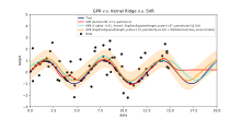
An example of Gaussian Process Regression (prediction) compared with other regression models.

A Gaussian process can be used as a prior probability distribution over functions in Bayesian inference. Given any set of N points in the desired domain of your functions, take a multivariate Gaussian whose covariance matrix parameter is the Gram matrix of your N points with some desired kernel, and sample from that Gaussian. For solution of the multi-output prediction problem, Gaussian process regression for vector-valued function was developed. In this method, a 'big' covariance is constructed, which describes the correlations between all the input and output variables taken in N points in the desired domain. This approach was elaborated in detail for the matrix-valued Gaussian processes and generalised to processes with 'heavier tails' like Student-t processes.

Inference of continuous values with a Gaussian process prior is known as Gaussian process regression, or kriging; extending Gaussian process regression to multiple target variables is known as cokriging. Gaussian processes are thus useful as a powerful non-linear multivariate interpolation tool.

Gaussian processes are also commonly used to tackle numerical analysis problems such as numerical integration, solving differential equations, or optimisation in the field of probabilistic numerics.

Gaussian processes can also be used in the context of mixture of experts models, for example. The underlying rationale of such a learning framework consists in the assumption that a given mapping cannot be well captured by a single Gaussian process model. Instead, the observation space is divided into subsets, each of which is characterized by a different mapping function; each of these is learned via a different Gaussian process component in the postulated mixture.

In the natural sciences, Gaussian processes have found use as probabilistic models of astronomical time series and as predictors of molecular properties.

Gaussian process prediction, or Kriging

Further information: Kriging

Gaussian Process Regression (prediction) with a squared exponential kernel. Left plot are draws from the prior function distribution. Middle are draws from the posterior. Right is mean prediction with one standard deviation shaded.

When concerned with a general Gaussian process regression problem (Kriging), it is assumed that for a Gaussian process ${\displaystyle f}$ observed at coordinates ${\displaystyle x}$, the vector of values ${\displaystyle f(x)}$ is just one sample from a multivariate Gaussian distribution of dimension equal to number of observed coordinates ${\displaystyle n}$. Therefore, under the assumption of a zero-mean distribution, ${\displaystyle f(x^{\prime })\sim N(0,K(\theta ,x,x^{\prime }))}$, where ${\displaystyle K(\theta ,x,x^{\prime })}$ is the covariance matrix between all possible pairs ${\displaystyle (x,x^{\prime })}$ for a given set of hyperparameters θ. As such the log marginal likelihood is:

$${\displaystyle \log p(f(x^{\prime })\mid \theta ,x)=-\frac{1}{2}\left(f(x{)}^{\mathsf{T}}K(\theta ,x,x^{\prime }{)}^{-1}f(x^{\prime })+\log det(K(\theta ,x,x^{\prime }))+n\log 2\pi \right)}$$

and maximizing this marginal likelihood towards θ provides the complete specification of the Gaussian process f. One can briefly note at this point that the first term corresponds to a penalty term for a model's failure to fit observed values and the second term to a penalty term that increases proportionally to a model's complexity. Having specified θ, making predictions about unobserved values ${\displaystyle f(x^{\ast })}$ at coordinates x* is then only a matter of drawing samples from the predictive distribution ${\displaystyle p(y^{\ast }\mid x^{\ast },f(x),x)=N(y^{\ast }\mid A,B)}$ where the posterior mean estimate A is defined as

$${\displaystyle A=K(\theta ,x^{\ast },x)K(\theta ,x,x^{\prime }{)}^{-1}f(x)}$$

and the posterior variance estimate B is defined as:

$${\displaystyle B=K(\theta ,x^{\ast },x^{\ast })-K(\theta ,x^{\ast },x)K(\theta ,x,x^{\prime }{)}^{-1}K(\theta ,x^{\ast },x{)}^{\mathsf{T}}}$$

where ${\displaystyle K(\theta ,x^{\ast },x)}$ is the covariance between the new coordinate of estimation x* and all other observed coordinates x for a given hyperparameter vector θ, ${\displaystyle K(\theta ,x,x^{\prime })}$ and ${\displaystyle f(x)}$ are defined as before and ${\displaystyle K(\theta ,x^{\ast },x^{\ast })}$ is the variance at point x* as dictated by θ. It is important to note that practically the posterior mean estimate of ${\displaystyle f(x^{\ast })}$ (the "point estimate") is just a linear combination of the observations ${\displaystyle f(x)}$; in a similar manner the variance of ${\displaystyle f(x^{\ast })}$ is actually independent of the observations ${\displaystyle f(x)}$. A known bottleneck in Gaussian process prediction is that the computational complexity of inference and likelihood evaluation is cubic in the number of points |x|, and as such can become unfeasible for larger data sets. Works on sparse Gaussian processes, that usually are based on the idea of building a representative set for the given process f, try to circumvent this issue. The kriging method can be used in the latent level of a nonlinear mixed-effects model for a spatial functional prediction: this technique is called the latent kriging.

Often, the covariance has the form $K(\theta ,x,x^{\prime })=\frac{1}{{\sigma }^2}\tilde{K}(\theta ,x,x^{\prime })$, where ${\displaystyle {\sigma }^2}$ is a scaling parameter. Examples are the Matérn class covariance functions. If this scaling parameter ${\displaystyle {\sigma }^2}$ is either known or unknown (i.e. must be marginalized), then the posterior probability, ${\displaystyle p(\theta \mid D)}$, i.e. the probability for the hyperparameters ${\displaystyle \theta }$ given a set of data pairs ${\displaystyle D}$ of observations of ${\displaystyle x}$ and ${\displaystyle f(x)}$, admits an analytical expression.

Bayesian neural networks as Gaussian processes

Further information: Neural network Gaussian process

Bayesian neural networks are a particular type of Bayesian network that results from treating deep learning and artificial neural network models probabilistically, and assigning a prior distribution to their parameters. Computation in artificial neural networks is usually organized into sequential layers of artificial neurons. The number of neurons in a layer is called the layer width. As layer width grows large, many Bayesian neural networks reduce to a Gaussian process with a closed form compositional kernel. This Gaussian process is called the Neural Network Gaussian Process (NNGP). It allows predictions from Bayesian neural networks to be more efficiently evaluated, and provides an analytic tool to understand deep learning models.

Computational issues

See also: Gaussian process approximations

In practical applications, Gaussian process models are often evaluated on a grid leading to multivariate normal distributions. Using these models for prediction or parameter estimation using maximum likelihood requires evaluating a multivariate Gaussian density, which involves calculating the determinant and the inverse of the covariance matrix. Both of these operations have cubic computational complexity which means that even for grids of modest sizes, both operations can have a prohibitive computational cost. This drawback led to the development of multiple approximation methods.