Search This Blog

Tuesday, February 20, 2024

Mathematical modelling of infectious diseases

From Wikipedia, the free encyclopedia

Mathematical models can project how infectious diseases progress to show the likely outcome of an epidemic (including in plants) and help inform public health and plant health interventions. Models use basic assumptions or collected statistics along with mathematics to find parameters for various infectious diseases and use those parameters to calculate the effects of different interventions, like mass vaccination programs. The modelling can help decide which intervention(s) to avoid and which to trial, or can predict future growth patterns, etc.

History

The modelling of infectious diseases is a tool that has been used to study the mechanisms by which diseases spread, to predict the future course of an outbreak and to evaluate strategies to control an epidemic.

The first scientist who systematically tried to quantify causes of death was John Graunt in his book Natural and Political Observations made upon the Bills of Mortality, in 1662. The bills he studied were listings of numbers and causes of deaths published weekly. Graunt's analysis of causes of death is considered the beginning of the "theory of competing risks" which according to Daley and Gani is "a theory that is now well established among modern epidemiologists".

The earliest account of mathematical modelling of spread of disease was carried out in 1760 by Daniel Bernoulli. Trained as a physician, Bernoulli created a mathematical model to defend the practice of inoculating against smallpox. The calculations from this model showed that universal inoculation against smallpox would increase the life expectancy from 26 years 7 months to 29 years 9 months. Daniel Bernoulli's work preceded the modern understanding of germ theory.

In the early 20th century, William Hamer and Ronald Ross applied the law of mass action to explain epidemic behaviour.

The 1920s saw the emergence of compartmental models. The Kermack–McKendrick epidemic model (1927) and the Reed–Frost epidemic model (1928) both describe the relationship between susceptible, infected and immune individuals in a population. The Kermack–McKendrick epidemic model was successful in predicting the behavior of outbreaks very similar to that observed in many recorded epidemics.

Recently, agent-based models (ABMs) have been used in exchange for simpler compartmental models. For example, epidemiological ABMs have been used to inform public health (nonpharmaceutical) interventions against the spread of SARS-CoV-2. Epidemiological ABMs, in spite of their complexity and requiring high computational power, have been criticized for simplifying and unrealistic assumptions. Still, they can be useful in informing decisions regarding mitigation and suppression measures in cases when ABMs are accurately calibrated.

Assumptions

Models are only as good as the assumptions on which they are based. If a model makes predictions that are out of line with observed results and the mathematics is correct, the initial assumptions must change to make the model useful.

  • Rectangular and stationary age distribution, i.e., everybody in the population lives to age L and then dies, and for each age (up to L) there is the same number of people in the population. This is often well-justified for developed countries where there is a low infant mortality and much of the population lives to the life expectancy.
  • Homogeneous mixing of the population, i.e., individuals of the population under scrutiny assort and make contact at random and do not mix mostly in a smaller subgroup. This assumption is rarely justified because social structure is widespread. For example, most people in London only make contact with other Londoners. Further, within London then there are smaller subgroups, such as the Turkish community or teenagers (just to give two examples), who mix with each other more than people outside their group. However, homogeneous mixing is a standard assumption to make the mathematics tractable.

Types of epidemic models

Stochastic

"Stochastic" means being or having a random variable. A stochastic model is a tool for estimating probability distributions of potential outcomes by allowing for random variation in one or more inputs over time. Stochastic models depend on the chance variations in risk of exposure, disease and other illness dynamics. Statistical agent-level disease dissemination in small or large populations can be determined by stochastic methods.

Deterministic

When dealing with large populations, as in the case of tuberculosis, deterministic or compartmental mathematical models are often used. In a deterministic model, individuals in the population are assigned to different subgroups or compartments, each representing a specific stage of the epidemic.

The transition rates from one class to another are mathematically expressed as derivatives, hence the model is formulated using differential equations. While building such models, it must be assumed that the population size in a compartment is differentiable with respect to time and that the epidemic process is deterministic. In other words, the changes in population of a compartment can be calculated using only the history that was used to develop the model.

Sub-exponential growth

A common explanation for the growth of epidemics holds that 1 person infects 2, those 2 infect 4 and so on and so on with the number of infected doubling every generation. It is analogous to a game of tag where 1 person tags 2, those 2 tag 4 others who've never been tagged and so on. As this game progresses it becomes increasing frenetic as the tagged run past the previously tagged to hunt down those who have never been tagged. Thus this model of an epidemic leads to a curve that grows exponentially until it crashes to zero as all the population have been infected. i.e. no herd immunity and no peak and gradual decline as seen in reality.

Reproduction number

The basic reproduction number (denoted by R0) is a measure of how transferable a disease is. It is the average number of people that a single infectious person will infect over the course of their infection. This quantity determines whether the infection will increase sub-exponentially, die out, or remain constant: if R0 > 1, then each person on average infects more than one other person so the disease will spread; if R0 < 1, then each person infects fewer than one person on average so the disease will die out; and if R0 = 1, then each person will infect on average exactly one other person, so the disease will become endemic: it will move throughout the population but not increase or decrease.

Endemic steady state

An infectious disease is said to be endemic when it can be sustained in a population without the need for external inputs. This means that, on average, each infected person is infecting exactly one other person (any more and the number of people infected will grow sub-exponentially and there will be an epidemic, any less and the disease will die out). In mathematical terms, that is:

The basic reproduction number (R0) of the disease, assuming everyone is susceptible, multiplied by the proportion of the population that is actually susceptible (S) must be one (since those who are not susceptible do not feature in our calculations as they cannot contract the disease). Notice that this relation means that for a disease to be in the endemic steady state, the higher the basic reproduction number, the lower the proportion of the population susceptible must be, and vice versa. This expression has limitations concerning the susceptibility proportion, e.g. the R0 equals 0.5 implicates S has to be 2, however this proportion exceeds the population size.

Assume the rectangular stationary age distribution and let also the ages of infection have the same distribution for each birth year. Let the average age of infection be A, for instance when individuals younger than A are susceptible and those older than A are immune (or infectious). Then it can be shown by an easy argument that the proportion of the population that is susceptible is given by:

We reiterate that L is the age at which in this model every individual is assumed to die. But the mathematical definition of the endemic steady state can be rearranged to give:

Therefore, due to the transitive property:

This provides a simple way to estimate the parameter R0 using easily available data.

For a population with an exponential age distribution,

This allows for the basic reproduction number of a disease given A and L in either type of population distribution.

Compartmental models in epidemiology

Compartmental models are formulated as Markov chains. A classic compartmental model in epidemiology is the SIR model, which may be used as a simple model for modelling epidemics. Multiple other types of compartmental models are also employed.

The SIR model

Diagram of the SIR model with initial values , and rates for infection and for recovery
Animation of the SIR model with initial values , and rate of recovery . The animation shows the effect of reducing the rate of infection from to . If there is no medicine or vaccination available, it is only possible to reduce the infection rate (often referred to as "flattening the curve") by appropriate measures such as social distancing.

In 1927, W. O. Kermack and A. G. McKendrick created a model in which they considered a fixed population with only three compartments: susceptible, ; infected, ; and recovered, . The compartments used for this model consist of three classes:

  • is used to represent the individuals not yet infected with the disease at time t, or those susceptible to the disease of the population.
  • denotes the individuals of the population who have been infected with the disease and are capable of spreading the disease to those in the susceptible category.
  • is the compartment used for the individuals of the population who have been infected and then removed from the disease, either due to immunization or due to death. Those in this category are not able to be infected again or to transmit the infection to others.

Other compartmental models

There are many modifications of the SIR model, including those that include births and deaths, where upon recovery there is no immunity (SIS model), where immunity lasts only for a short period of time (SIRS), where there is a latent period of the disease where the person is not infectious (SEIS and SEIR), and where infants can be born with immunity (MSIR).

Infectious disease dynamics

Mathematical models need to integrate the increasing volume of data being generated on host-pathogen interactions. Many theoretical studies of the population dynamics, structure and evolution of infectious diseases of plants and animals, including humans, are concerned with this problem.

Research topics include:

Mathematics of mass vaccination

If the proportion of the population that is immune exceeds the herd immunity level for the disease, then the disease can no longer persist in the population and its transmission dies out. Thus, a disease can be eliminated from a population if enough individuals are immune due to either vaccination or recovery from prior exposure to disease. For example, smallpox eradication, with the last wild case in 1977, and certification of the eradication of indigenous transmission of 2 of the 3 types of wild poliovirus (type 2 in 2015, after the last reported case in 1999, and type 3 in 2019, after the last reported case in 2012).

The herd immunity level will be denoted q. Recall that, for a stable state:

In turn,

which is approximately:
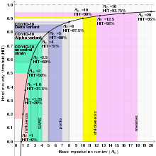
Graph of herd immunity threshold vs basic reproduction number with selected diseases

S will be (1 − q), since q is the proportion of the population that is immune and q + S must equal one (since in this simplified model, everyone is either susceptible or immune). Then:

Remember that this is the threshold level. Die out of transmission will only occur if the proportion of immune individuals exceeds this level due to a mass vaccination programme.

We have just calculated the critical immunization threshold (denoted qc). It is the minimum proportion of the population that must be immunized at birth (or close to birth) in order for the infection to die out in the population.

Because the fraction of the final size of the population p that is never infected can be defined as:

Hence,

Solving for , we obtain:

When mass vaccination cannot exceed the herd immunity

If the vaccine used is insufficiently effective or the required coverage cannot be reached, the program may fail to exceed qc. Such a program will protect vaccinated individuals from disease, but may change the dynamics of transmission.

Suppose that a proportion of the population q (where q < qc) is immunised at birth against an infection with R0 > 1. The vaccination programme changes R0 to Rq where

This change occurs simply because there are now fewer susceptibles in the population who can be infected. Rq is simply R0 minus those that would normally be infected but that cannot be now since they are immune.

As a consequence of this lower basic reproduction number, the average age of infection A will also change to some new value Aq in those who have been left unvaccinated.

Recall the relation that linked R0, A and L. Assuming that life expectancy has not changed, now:

But R0 = L/A so:

Thus, the vaccination program may raise the average age of infection, and unvaccinated individuals will experience a reduced force of infection due to the presence of the vaccinated group. For a disease that leads to greater clinical severity in older populations, the unvaccinated proportion of the population may experience the disease relatively later in life than would occur in the absence of vaccine.

When mass vaccination exceeds the herd immunity

If a vaccination program causes the proportion of immune individuals in a population to exceed the critical threshold for a significant length of time, transmission of the infectious disease in that population will stop. If elimination occurs everywhere at the same time, then this can lead to eradication.

Elimination
Interruption of endemic transmission of an infectious disease, which occurs if each infected individual infects less than one other, is achieved by maintaining vaccination coverage to keep the proportion of immune individuals above the critical immunization threshold.
Eradication
Elimination everywhere at the same time such that the infectious agent dies out (for example, smallpox and rinderpest).

Reliability

Models have the advantage of examining multiple outcomes simultaneously, rather than making a single forecast. Models have shown broad degrees of reliability in past pandemics, such as SARS, SARS-CoV-2, Swine flu, MERS and Ebola.

Mathematical model

From Wikipedia, the free encyclopedia

A mathematical model is an abstract description of a concrete system using mathematical concepts and language. The process of developing a mathematical model is termed mathematical modeling. Mathematical models are used in applied mathematics and in the natural sciences (such as physics, biology, earth science, chemistry) and engineering disciplines (such as computer science, electrical engineering), as well as in non-physical systems such as the social sciences (such as economics, psychology, sociology, political science). It can also be taught as a subject in its own right.

The use of mathematical models to solve problems in business or military operations is a large part of the field of operations research.

Mathematical models are also used in music, linguistics, and philosophy (for example, intensively in analytic philosophy). A model may help to explain a system and to study the effects of different components, and to make predictions about behavior.

Elements of a mathematical model

Mathematical models can take many forms, including dynamical systems, statistical models, differential equations, or game theoretic models. These and other types of models can overlap, with a given model involving a variety of abstract structures. In general, mathematical models may include logical models. In many cases, the quality of a scientific field depends on how well the mathematical models developed on the theoretical side agree with results of repeatable experiments. Lack of agreement between theoretical mathematical models and experimental measurements often leads to important advances as better theories are developed.

In the physical sciences, a traditional mathematical model contains most of the following elements:

  1. Governing equations
  2. Supplementary sub-models
    1. Defining equations
    2. Constitutive equations
  3. Assumptions and constraints
    1. Initial and boundary conditions
    2. Classical constraints and kinematic equations

Classifications

Mathematical models are of different types:

  • Linear vs. nonlinear: If all the operators in a mathematical model exhibit linearity, the resulting mathematical model is defined as linear. A model is considered to be nonlinear otherwise. The definition of linearity and nonlinearity is dependent on context, and linear models may have nonlinear expressions in them. For example, in a statistical linear model, it is assumed that a relationship is linear in the parameters, but it may be nonlinear in the predictor variables. Similarly, a differential equation is said to be linear if it can be written with linear differential operators, but it can still have nonlinear expressions in it. In a mathematical programming model, if the objective functions and constraints are represented entirely by linear equations, then the model is regarded as a linear model. If one or more of the objective functions or constraints are represented with a nonlinear equation, then the model is known as a nonlinear model.
    Linear structure implies that a problem can be decomposed into simpler parts that can be treated independently and/or analyzed at a different scale and the results obtained will remain valid for the initial problem when recomposed and rescaled.
    Nonlinearity, even in fairly simple systems, is often associated with phenomena such as chaos and irreversibility. Although there are exceptions, nonlinear systems and models tend to be more difficult to study than linear ones. A common approach to nonlinear problems is linearization, but this can be problematic if one is trying to study aspects such as irreversibility, which are strongly tied to nonlinearity.
  • Static vs. dynamic: A dynamic model accounts for time-dependent changes in the state of the system, while a static (or steady-state) model calculates the system in equilibrium, and thus is time-invariant. Dynamic models typically are represented by differential equations or difference equations.
  • Explicit vs. implicit: If all of the input parameters of the overall model are known, and the output parameters can be calculated by a finite series of computations, the model is said to be explicit. But sometimes it is the output parameters which are known, and the corresponding inputs must be solved for by an iterative procedure, such as Newton's method or Broyden's method. In such a case the model is said to be implicit. For example, a jet engine's physical properties such as turbine and nozzle throat areas can be explicitly calculated given a design thermodynamic cycle (air and fuel flow rates, pressures, and temperatures) at a specific flight condition and power setting, but the engine's operating cycles at other flight conditions and power settings cannot be explicitly calculated from the constant physical properties.
  • Discrete vs. continuous: A discrete model treats objects as discrete, such as the particles in a molecular model or the states in a statistical model; while a continuous model represents the objects in a continuous manner, such as the velocity field of fluid in pipe flows, temperatures and stresses in a solid, and electric field that applies continuously over the entire model due to a point charge.
  • Deterministic vs. probabilistic (stochastic): A deterministic model is one in which every set of variable states is uniquely determined by parameters in the model and by sets of previous states of these variables; therefore, a deterministic model always performs the same way for a given set of initial conditions. Conversely, in a stochastic model—usually called a "statistical model"—randomness is present, and variable states are not described by unique values, but rather by probability distributions.
  • Deductive, inductive, or floating: A deductive model is a logical structure based on a theory. An inductive model arises from empirical findings and generalization from them. The floating model rests on neither theory nor observation, but is merely the invocation of expected structure. Application of mathematics in social sciences outside of economics has been criticized for unfounded models. Application of catastrophe theory in science has been characterized as a floating model.
  • Strategic vs non-strategic Models used in game theory are different in a sense that they model agents with incompatible incentives, such as competing species or bidders in an auction. Strategic models assume that players are autonomous decision makers who rationally choose actions that maximize their objective function. A key challenge of using strategic models is defining and computing solution concepts such as Nash equilibrium. An interesting property of strategic models is that they separate reasoning about rules of the game from reasoning about behavior of the players.

Construction

In business and engineering, mathematical models may be used to maximize a certain output. The system under consideration will require certain inputs. The system relating inputs to outputs depends on other variables too: decision variables, state variables, exogenous variables, and random variables.

Decision variables are sometimes known as independent variables. Exogenous variables are sometimes known as parameters or constants. The variables are not independent of each other as the state variables are dependent on the decision, input, random, and exogenous variables. Furthermore, the output variables are dependent on the state of the system (represented by the state variables).

Objectives and constraints of the system and its users can be represented as functions of the output variables or state variables. The objective functions will depend on the perspective of the model's user. Depending on the context, an objective function is also known as an index of performance, as it is some measure of interest to the user. Although there is no limit to the number of objective functions and constraints a model can have, using or optimizing the model becomes more involved (computationally) as the number increases.

For example, economists often apply linear algebra when using input–output models. Complicated mathematical models that have many variables may be consolidated by use of vectors where one symbol represents several variables.

A priori information

To analyse something with a typical "black box approach", only the behavior of the stimulus/response will be accounted for, to infer the (unknown) box. The usual representation of this black box system is a data flow diagram centered in the box.

Mathematical modeling problems are often classified into black box or white box models, according to how much a priori information on the system is available. A black-box model is a system of which there is no a priori information available. A white-box model (also called glass box or clear box) is a system where all necessary information is available. Practically all systems are somewhere between the black-box and white-box models, so this concept is useful only as an intuitive guide for deciding which approach to take.

Usually, it is preferable to use as much a priori information as possible to make the model more accurate. Therefore, the white-box models are usually considered easier, because if you have used the information correctly, then the model will behave correctly. Often the a priori information comes in forms of knowing the type of functions relating different variables. For example, if we make a model of how a medicine works in a human system, we know that usually the amount of medicine in the blood is an exponentially decaying function. But we are still left with several unknown parameters; how rapidly does the medicine amount decay, and what is the initial amount of medicine in blood? This example is therefore not a completely white-box model. These parameters have to be estimated through some means before one can use the model.

In black-box models, one tries to estimate both the functional form of relations between variables and the numerical parameters in those functions. Using a priori information we could end up, for example, with a set of functions that probably could describe the system adequately. If there is no a priori information we would try to use functions as general as possible to cover all different models. An often used approach for black-box models are neural networks which usually do not make assumptions about incoming data. Alternatively, the NARMAX (Nonlinear AutoRegressive Moving Average model with eXogenous inputs) algorithms which were developed as part of nonlinear system identification can be used to select the model terms, determine the model structure, and estimate the unknown parameters in the presence of correlated and nonlinear noise. The advantage of NARMAX models compared to neural networks is that NARMAX produces models that can be written down and related to the underlying process, whereas neural networks produce an approximation that is opaque.

Subjective information

Sometimes it is useful to incorporate subjective information into a mathematical model. This can be done based on intuition, experience, or expert opinion, or based on convenience of mathematical form. Bayesian statistics provides a theoretical framework for incorporating such subjectivity into a rigorous analysis: we specify a prior probability distribution (which can be subjective), and then update this distribution based on empirical data.

An example of when such approach would be necessary is a situation in which an experimenter bends a coin slightly and tosses it once, recording whether it comes up heads, and is then given the task of predicting the probability that the next flip comes up heads. After bending the coin, the true probability that the coin will come up heads is unknown; so the experimenter would need to make a decision (perhaps by looking at the shape of the coin) about what prior distribution to use. Incorporation of such subjective information might be important to get an accurate estimate of the probability.

Complexity

In general, model complexity involves a trade-off between simplicity and accuracy of the model. Occam's razor is a principle particularly relevant to modeling, its essential idea being that among models with roughly equal predictive power, the simplest one is the most desirable. While added complexity usually improves the realism of a model, it can make the model difficult to understand and analyze, and can also pose computational problems, including numerical instability. Thomas Kuhn argues that as science progresses, explanations tend to become more complex before a paradigm shift offers radical simplification.

For example, when modeling the flight of an aircraft, we could embed each mechanical part of the aircraft into our model and would thus acquire an almost white-box model of the system. However, the computational cost of adding such a huge amount of detail would effectively inhibit the usage of such a model. Additionally, the uncertainty would increase due to an overly complex system, because each separate part induces some amount of variance into the model. It is therefore usually appropriate to make some approximations to reduce the model to a sensible size. Engineers often can accept some approximations in order to get a more robust and simple model. For example, Newton's classical mechanics is an approximated model of the real world. Still, Newton's model is quite sufficient for most ordinary-life situations, that is, as long as particle speeds are well below the speed of light, and we study macro-particles only.

Note that better accuracy does not necessarily mean a better model. Statistical models are prone to overfitting which means that a model is fitted to data too much and it has lost its ability to generalize to new events that were not observed before.

Training, tuning, and fitting

Any model which is not pure white-box contains some parameters that can be used to fit the model to the system it is intended to describe. If the modeling is done by an artificial neural network or other machine learning, the optimization of parameters is called training, while the optimization of model hyperparameters is called tuning and often uses cross-validation. In more conventional modeling through explicitly given mathematical functions, parameters are often determined by curve fitting.

Evaluation and assessment

A crucial part of the modeling process is the evaluation of whether or not a given mathematical model describes a system accurately. This question can be difficult to answer as it involves several different types of evaluation.

Prediction of empirical data

Usually, the easiest part of model evaluation is checking whether a model predicts experimental measurements or other empirical data not used in the model development. In models with parameters, a common approach is to split the data into two disjoint subsets: training data and verification data. The training data are used to estimate the model parameters. An accurate model will closely match the verification data even though these data were not used to set the model's parameters. This practice is referred to as cross-validation in statistics.

Defining a metric to measure distances between observed and predicted data is a useful tool for assessing model fit. In statistics, decision theory, and some economic models, a loss function plays a similar role.

While it is rather straightforward to test the appropriateness of parameters, it can be more difficult to test the validity of the general mathematical form of a model. In general, more mathematical tools have been developed to test the fit of statistical models than models involving differential equations. Tools from nonparametric statistics can sometimes be used to evaluate how well the data fit a known distribution or to come up with a general model that makes only minimal assumptions about the model's mathematical form.

Scope of the model

Assessing the scope of a model, that is, determining what situations the model is applicable to, can be less straightforward. If the model was constructed based on a set of data, one must determine for which systems or situations the known data is a "typical" set of data.

The question of whether the model describes well the properties of the system between data points is called interpolation, and the same question for events or data points outside the observed data is called extrapolation.

As an example of the typical limitations of the scope of a model, in evaluating Newtonian classical mechanics, we can note that Newton made his measurements without advanced equipment, so he could not measure properties of particles traveling at speeds close to the speed of light. Likewise, he did not measure the movements of molecules and other small particles, but macro particles only. It is then not surprising that his model does not extrapolate well into these domains, even though his model is quite sufficient for ordinary life physics.

Philosophical considerations

Many types of modeling implicitly involve claims about causality. This is usually (but not always) true of models involving differential equations. As the purpose of modeling is to increase our understanding of the world, the validity of a model rests not only on its fit to empirical observations, but also on its ability to extrapolate to situations or data beyond those originally described in the model. One can think of this as the differentiation between qualitative and quantitative predictions. One can also argue that a model is worthless unless it provides some insight which goes beyond what is already known from direct investigation of the phenomenon being studied.

An example of such criticism is the argument that the mathematical models of optimal foraging theory do not offer insight that goes beyond the common-sense conclusions of evolution and other basic principles of ecology.

It should also be noted that while mathematical modeling uses mathematical concepts and language, it is not itself a branch of mathematics and does not necessarily conform to any mathematical logic, but is typically a branch of some science or other technical subject, with corresponding concepts and standards of argumentation.

Significance in the natural sciences

Mathematical models are of great importance in the natural sciences, particularly in physics. Physical theories are almost invariably expressed using mathematical models.

Throughout history, more and more accurate mathematical models have been developed. Newton's laws accurately describe many everyday phenomena, but at certain limits theory of relativity and quantum mechanics must be used.

It is common to use idealized models in physics to simplify things. Massless ropes, point particles, ideal gases and the particle in a box are among the many simplified models used in physics. The laws of physics are represented with simple equations such as Newton's laws, Maxwell's equations and the Schrödinger equation. These laws are a basis for making mathematical models of real situations. Many real situations are very complex and thus modeled approximately on a computer, a model that is computationally feasible to compute is made from the basic laws or from approximate models made from the basic laws. For example, molecules can be modeled by molecular orbital models that are approximate solutions to the Schrödinger equation. In engineering, physics models are often made by mathematical methods such as finite element analysis.

Different mathematical models use different geometries that are not necessarily accurate descriptions of the geometry of the universe. Euclidean geometry is much used in classical physics, while special relativity and general relativity are examples of theories that use geometries which are not Euclidean.

Some applications

Often when engineers analyze a system to be controlled or optimized, they use a mathematical model. In analysis, engineers can build a descriptive model of the system as a hypothesis of how the system could work, or try to estimate how an unforeseeable event could affect the system. Similarly, in control of a system, engineers can try out different control approaches in simulations.

A mathematical model usually describes a system by a set of variables and a set of equations that establish relationships between the variables. Variables may be of many types; real or integer numbers, Boolean values or strings, for example. The variables represent some properties of the system, for example, the measured system outputs often in the form of signals, timing data, counters, and event occurrence. The actual model is the set of functions that describe the relations between the different variables.

Examples

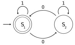
  • One of the popular examples in computer science is the mathematical models of various machines, an example is the deterministic finite automaton (DFA) which is defined as an abstract mathematical concept, but due to the deterministic nature of a DFA, it is implementable in hardware and software for solving various specific problems. For example, the following is a DFA M with a binary alphabet, which requires that the input contains an even number of 0s:
The state diagram for
where
  • and
  • is defined by the following state-transition table:

0
1
S1
S2
The state represents that there has been an even number of 0s in the input so far, while signifies an odd number. A 1 in the input does not change the state of the automaton. When the input ends, the state will show whether the input contained an even number of 0s or not. If the input did contain an even number of 0s, will finish in state an accepting state, so the input string will be accepted.
The language recognized by is the regular language given by the regular expression 1*( 0 (1*) 0 (1*) )*, where "*" is the Kleene star, e.g., 1* denotes any non-negative number (possibly zero) of symbols "1".
  • Many everyday activities carried out without a thought are uses of mathematical models. A geographical map projection of a region of the earth onto a small, plane surface is a model which can be used for many purposes such as planning travel.
  • Another simple activity is predicting the position of a vehicle from its initial position, direction and speed of travel, using the equation that distance traveled is the product of time and speed. This is known as dead reckoning when used more formally. Mathematical modeling in this way does not necessarily require formal mathematics; animals have been shown to use dead reckoning.
  • Population Growth. A simple (though approximate) model of population growth is the Malthusian growth model. A slightly more realistic and largely used population growth model is the logistic function, and its extensions.
  • Model of a particle in a potential-field. In this model we consider a particle as being a point of mass which describes a trajectory in space which is modeled by a function giving its coordinates in space as a function of time. The potential field is given by a function and the trajectory, that is a function is the solution of the differential equation:
    that can be written also as
Note this model assumes the particle is a point mass, which is certainly known to be false in many cases in which we use this model; for example, as a model of planetary motion.
  • Model of rational behavior for a consumer. In this model we assume a consumer faces a choice of commodities labeled each with a market price The consumer is assumed to have an ordinal utility function (ordinal in the sense that only the sign of the differences between two utilities, and not the level of each utility, is meaningful), depending on the amounts of commodities consumed. The model further assumes that the consumer has a budget which is used to purchase a vector in such a way as to maximize The problem of rational behavior in this model then becomes a mathematical optimization problem, that is:
    subject to:
    This model has been used in a wide variety of economic contexts, such as in general equilibrium theory to show existence and Pareto efficiency of economic equilibria.
  • Neighbour-sensing model is a model that explains the mushroom formation from the initially chaotic fungal network.
  • In computer science, mathematical models may be used to simulate computer networks.
  • In mechanics, mathematical models may be used to analyze the movement of a rocket model.

Truth Decay (book)

From Wikipedia, the free encyclopedia
 
Truth Decay
AuthorJennifer Kavanagh and Michael Rich
CountryUnited States
LanguageEnglish
GenreNon-fiction
PublisherRAND Corporation
Publication date
January 16, 2018

Truth Decay is a non-fiction book by Jennifer Kavanagh and Michael D. Rich. Published by the RAND Corporation on January 16, 2018, the book examines historical trends such as "yellow journalism" and "new journalism" to demonstrate that "truth decay" is not a new phenomenon in American society. The authors argue that the divergence between individuals over objective facts and the concomitant increase in the relative "volume and influence of opinion over fact" in civil and political discourse has historically proliferated American society and culminated in truth decay.

The term "truth decay" was suggested by Sonni Efron and adopted by the authors of the book to characterize four interrelated trends in American society.

Kavanagh and Rich describe the "drivers" of truth decay as cognitive prejudices, transformation of information systems, competing demands on the education system, and polarization. This has consequences on various aspects of American society. The authors argue that truth decay has engendered the deterioration of "civil discourse" and "politica paralysis". This has culminated in an increasing withdrawal of individuals from institutional sites of discourse throughout modern American society.

Truth Decay was positively received by audiences. The book was a nonfiction bestseller in the United States. Indeed, Barack Obama included the "very interesting" book in his 2018 reading list. Further, it stimulated a panel discussion at the University of Sydney on the role of media institutions in society and the ways in which democratic governance and civic engagement can be improved.

Publishing history

Truth Decay was first published as a web-only book on January 16, 2018, by the RAND corporation. This allowed individuals to read the book online without incurring any costs. On 26 January 2018, physical copies of the book were also published by the RAND corporation and made available for order on websites such as Amazon and Apple Books.

The RAND corporation is a non-profit and nonpartisan research organization that is based in California.[8] It is concerned about the social, economic and political dangers that truth decay poses to the decision making processes of individuals in society. Kavanagh, a senior political scientist, has expressed concern that there is an increasing number of people in America and Europe are doubtful of climate change and the efficacy of vaccines.

The term truth decay

In Chapter 1, Kavanagh and Rich introduce the term “truth decay”. The term “truth decay” was suggested by Sonni Efron and adopted by the authors of the book to characterize four interrelated trends in American society, including:

  • Increasing differences between individuals about objective facts;
  • Increasing conflation of opinion and fact in discourse;
  • Increasing quantity and authority of opinion rather than fact in discourse; and
  • Diminishing faith in traditionally authoritative sources of reliable and accurate information.

Kavanagh and Rich differentiate truth decay from “fake news”. The authors argue that phenomena such as “fake news” have not, in themselves, catalyzed the shift away from objective facts in political and civil discourse. The authors allege that “fake news” constitutes an aspect of truth decay and the associated challenges arising from the diminishing faith in historically authoritative sources of accurate information such as government, media and education. Notwithstanding this distinction, the authors argue that the expression “fake news” has been intentionally deployed by politicians such as Donald Trump and Vladimir Putin to diminish the accuracy and facticity of information promulgated by sources that do not align with their partisan position. In that context, the authors argue that a limited focus on phenomena such as “fake news” inhibits a vigorous analysis of the causes and consequences of truth decay in society.

Structure and major arguments

Truth Decay is organized in six chapters and explores three historical eras — the 1890s, 1920s, and 1960s — for historical evidence of the four trends of Truth Decay. The authors argue that Truth Decay is “not a new phenomenon” as there has been a sustained increase in the volume and influence of opinion over fact throughout the last century.

Historical context

In Chapter 3, the book explores three eras — the 1890s, 1920s, and 1960s — for historical evidence of the aforementioned four trends of truth decay in American society.

Gilded Age

Depiction of a young woman being strip-searched by imposing Spanish policemen (Illustrator: Frederic Remington)

First, the authors identify the 1880s–1890s as the "Gilded Age". This historical era commenced after the American Civil War and was punctuated by the industrialization of America. The introduction of printing technology increased the output of newspaper publishers. This stimulated competition within the newspaper publishing industry. In New York City, major newspaper publishers Joseph Pulitzer and William Hearst engaged in "yellow journalism" by deploying a sensationalist style of covering politics, world events and crime in order to fend off competitors and attract market share. The authors note that these publishers also deployed "yellow journalism" to advance the partisan political objectives of their respective news organizations. For example, in April 1898, the New York Journal owned by Hearst published a number of articles with bold headlines, violent images and aggrandized information to position the Cubans as "innocent" people being "persecuted by the illiberal Spanish" regime and thereby emphasize the propriety of America's intervention in the Spanish-American War to the audience. Thus, "yellow journalism" caused a conflation of opinions and objectively verifiable facts in society.

Roaring Twenties and the Great Depression

Second, the authors identify the 1920s–1930s as the Roaring Twenties and the Great Depression. This historical era was renowned as another period of economic growth and development that catalysed significant changes in the American media industry. The authors argue that radio broadcasting and tabloid journalism emerged as a dramatized form of media that focused on news surrounding public figures such as politicians, actors, musicians and sports athletes as entertainment rather than reliable and accurate information for the audience to utilise in considered decision-making. As such, "jazz journalism" is alleged to have amplified the conflation of opinions and objectively verifiable facts in society.

The Civil Rights Movement

Third, the authors identify the 1960s–1970s as the period of "civil rights and social unrest". This historical era was punctuated by America's involvement in the Vietnam War. Television news was used to disseminate information which portrayed the appropriateness and success of America's involvement in the Vietnam War to the audience. Kavanagh and Rich argue that this increasingly conflated opinion and objective facts to advance partisan objectives. The Civil Rights movement in the 1960s contributed to a transformation in news reporting. Journalists began to deploy first-person narration in their reporting of world events to illuminate the inequities faced by African American citizens who strived for recognition and civil rights. On its face, this incidence of "new journalism" increased the risk of reporters imbuing their work with personal biases. Nonetheless, Bainer suggests that "new journalism" also augmented reporting as it permitted journalists to disseminate information on matters without the hollow pretence of objective reporting.

Current drivers

In Chapter 4, Kavanagh and Rich describe the "drivers" of the aforementioned four trends of truth decay as cognitive prejudices, transformation of information systems and cuts to the education sector.

Cognitive prejudices

First, cognitive prejudices are described as systematic errors in rational thinking that transpire when individuals are absorbing information. Confirmation bias is the propensity to identify and prioritise information that supports a pre-existing worldview. This has a number of impacts on the process of individual decision-making. The authors argue that individuals consciously or unconsciously employ motivated reasoning to resist accepting information that challenges their pre-existing worldview. This causes the interface with invalidating information to further ingrain the partisan opinions of individuals. It is alleged by the authors that, in the long term, cognitive prejudices have created "political, sociodemographic, and economic polarisation" as individuals form cliques that are diametrically opposed in their worldview and communication, thereby attenuating the quality civil discourse in American society.

Transformation of information systems

Second, the transformation of information systems refers to the surge in the "volume and speed of news" that is disseminated to individuals. The authors note that the move towards a "24-hour news cycle" has increased the number of competitors to traditional news organizations. This competition, it is said, has reduced profitability and compelled news organizations such as ABC and Fox to pivot from costly investigative journalism to sensationalized opinion as a less-costly method of attracting an audience. The increase in the quantity of opinion rather than objectively discernible fact in reporting is further exacerbated by the introduction of social media platforms such as Twitter and Facebook. These social media platforms facilitate rapid access to, and dissemination of, opinion news to millions of users.

Cuts to the educational sector

U.S. Federal Budget Deficit from 2018 to 2027

Third, the authors allege that cuts to the educational sector have catalyzed a reduction in the critical thinking and media literacy education of individuals. Kavanagh and Rich argue that individuals utilise the information and critical thinking skills established in traditionally authoritative sites of discourse such as secondary schools and universities to make decisions. Financial constraints associated with the swelling federal budget deficit from 2010 to 2021 have precipitated cuts to the funding apportioned to the American education sector. The authors argue that this has meant that, in the face of the increasing volume of online news, fewer students have acquired the technical and emotional skills to identify the explicit and implicit biases of reporters and thereby critically assess the accuracy and reliability of information emanating from sources such as the government and media. Ranschaert uses data gained through a longitudinal study of social studies teachers to argue that the decline in individuals relying on teachers for authoritative information has serious implications for ability of the education system to act as a buffer against truth decay. The authors go further than Ranschaert by arguing that, in the long term, this has resulted in a constituency that is vulnerable to absorbing and promoting misinformation as the skill to delineate objective facts from misinformation has atrophied. In that context, the disparity between the media literacy education of students and the challenges posed by Internet technology is said to engender truth decay.

Current consequences

In Chapter 5, Kavanagh and Rich describe the consequences of truth decay in America.

Deterioration of civil discourse in society

Violent protests at the Minnesota Capitol

First, it is alleged that truth decay manifests in the deterioration of civil discourse in modern American society. The authors define civil discourse as vigorous dialogue that attempts to promote the public interest. It follows that, in the absence of a baseline set of objective facts, the authors suggest that the ability for individuals and politicians to meaningfully listen and engage in a constructive dialogue about economics, science and policy is diminished.

Political paralysis

Second, truth decay is alleged to manifest in "political paralysis". The authors note that the deterioration of civil discourse and increasing dispute about objective facts has created a deep chasm between conservative and liberal politicians in America. A case study on the increasing use of the filibuster in the United States Senate between 1947 and 2017 is used to suggest that truth decay has culminated in conservative and liberal politicians being increasingly unable to compromise on a range of policy initiatives. This incurs short term economic costs for the U.S. economy as the government becomes rigid an unable to respond promptly to domestic crises that require direct intervention. For example, America's federal government shut down in 2013 due to the inability of the Senate to pass the Affordable Care Act. The lack of funding for federal operations resulted in a $24 billion loss to the economy. In the long term, political paralysis also causes the U.S. to drop in international standing.

Withdrawal of individuals from institutional sites of discourse

Third, truth decay is alleged to have engendered the withdrawal of individuals from institutional sites of discourse. The authors argue that the decrease of faith in education institutions, media and government among young voters aged between 18 and 29 precipitated the consistent decrease in the overall number of votes cast in the U.S federal election from 2004 to 2016. This decrease in the exercise of civic responsibility through voting may, in the long run, diminish the ability of citizens to scrutinise state power, thereby diminishing policy making and overall accountability.

Reception

Truth Decay was positively received by American audiences. The book debuted as a Nonfiction Bestseller in 2018. On Amazon.com, the book is rated 4.3 stars out of 5 stars.

The book subsequently stimulated a panel discussion at the University of Sydney. On 22 August 2018, Michael Rich joined Professor Simon Jackman, John Barron, Nick Enfield and Lisa Bero for a discussion of the causes and consequences of truth decay in modern society. This panel was co-hosted by the RAND Australia and the United States Studies Centre.

Excerpts from the book were published by CNN, ABC and the Washington Post. An article on the ABC website reported on the "troubling trend" of truth decay which was "exposed" by the authors of the book.

Barack Obama included the "very interesting" book in his 2018 summer reading list. Obama noted that "a selective sorting of facts and evidence" is deceitful and corrosive to civil discourse. This is because "society has always worked best when reasoned debate and practical problem-solving thrive". This notion was echoed by Cãtãlina Nastasiu, who lauded the "ambitious exploratory work" because it "serves as a base to better understand the information ecosystem".

Computer-aided software engineering

From Wikipedia, the free encyclopedia ...