Faraday's law of induction

From Wikipedia, the free encyclopedia

Faraday's law of induction is a basic law of electromagnetism predicting how a magnetic field will interact with an electric circuit to produce an electromotive force (EMF)—a phenomenon called electromagnetic induction. It is the fundamental operating principle of transformers, inductors, and many types of electrical motors, generators and solenoids.^[1][2]

The Maxwell–Faraday equation is a generalization of Faraday's law, and is listed as one of Maxwell's equations.

History

A diagram of Faraday's iron ring apparatus. The changing magnetic flux of the left coil induces a current in the right coil.^[3]

 

Faraday's disk, the first electric generator, a type of homopolar generator.

Electromagnetic induction was discovered independently by Michael Faraday in 1831 and Joseph Henry in 1832.^[4] Faraday was the first to publish the results of his experiments.^[5][6] In Faraday's first experimental demonstration of electromagnetic induction (August 29, 1831),^[7] he wrapped two wires around opposite sides of an iron ring (torus) (an arrangement similar to a modern toroidal transformer). Based on his assessment of recently discovered properties of electromagnets, he expected that when current started to flow in one wire, a sort of wave would travel through the ring and cause some electrical effect on the opposite side. He plugged one wire into a galvanometer, and watched it as he connected the other wire to a battery. Indeed, he saw a transient current (which he called a "wave of electricity") when he connected the wire to the battery, and another when he disconnected it.^[8] This induction was due to the change in magnetic flux that occurred when the battery was connected and disconnected.^[3] Within two months, Faraday had found several other manifestations of electromagnetic induction. For example, he saw transient currents when he quickly slid a bar magnet in and out of a coil of wires, and he generated a steady (DC) current by rotating a copper disk near the bar magnet with a sliding electrical lead ("Faraday's disk").^[9]

Michael Faraday explained electromagnetic induction using a concept he called lines of force. However, scientists at the time widely rejected his theoretical ideas, mainly because they were not formulated mathematically.^[10] An exception was James Clerk Maxwell, who in 1861-2 used Faraday's ideas as the basis of his quantitative electromagnetic theory.^[10][11][12] In Maxwell's papers, the time-varying aspect of electromagnetic induction is expressed as a differential equation which Oliver Heaviside referred to as Faraday's law even though it is different from the original version of Faraday's law, and does not describe motional EMF. Heaviside's version (see Maxwell–Faraday equation below) is the form recognized today in the group of equations known as Maxwell's equations.

Lenz's law, formulated by Emil Lenz in 1834,^[13] describes "flux through the circuit", and gives the direction of the induced EMF and current resulting from electromagnetic induction (elaborated upon in the examples below).

Faraday's experiment showing induction between coils of wire: The liquid battery (right) provides a current which flows through the small coil (A), creating a magnetic field. When the coils are stationary, no current is induced. But when the small coil is moved in or out of the large coil (B), the magnetic flux through the large coil changes, inducing a current which is detected by the galvanometer (G).^[14]

Faraday's law

Qualitative statement

The most widespread version of Faraday's law states:

The induced electromotive force in any closed circuit is equal to the negative of the time rate of change of the magnetic flux enclosed by the circuit.^[15][16]

This version of Faraday's law strictly holds only when the closed circuit is a loop of infinitely thin wire,^[17] and is invalid in other circumstances as discussed below. A different version, the Maxwell–Faraday equation (discussed below), is valid in all circumstances.

Quantitative

The definition of surface integral relies on splitting the surface Σ into small surface elements. Each element is associated with a vector dA of magnitude equal to the area of the element and with direction normal to the element and pointing "outward" (with respect to the orientation of the surface).

Faraday's law of induction makes use of the magnetic flux Φ_B through a hypothetical surface Σ whose boundary is a wire loop. Since the wire loop may be moving, we write Σ(t) for the surface. The magnetic flux is defined by a surface integral:

${\displaystyle \Phi _{B}=\iint \limits _{\Sigma (t)}\mathbf {B} (\mathbf {r} ,t)\cdot d\mathbf {A} \,,}$

where dA is an element of surface area of the moving surface Σ(t), B is the magnetic field (also called "magnetic flux density"), and B·dA is a vector dot product (the infinitesimal amount of magnetic flux through the infinitesimal area element dA). In more visual terms, the magnetic flux through the wire loop is proportional to the number of magnetic flux lines that pass through the loop.

When the flux changes—because B changes, or because the wire loop is moved or deformed, or both—Faraday's law of induction says that the wire loop acquires an EMF, ℰ, defined as the energy available from a unit charge that has travelled once around the wire loop.^{[17][18][19][20]} Equivalently, it is the voltage that would be measured by cutting the wire to create an open circuit, and attaching a voltmeter to the leads.

Faraday's law states that the EMF is also given by the rate of change of the magnetic flux:

${\displaystyle {\mathcal {E}}=-{\frac {d\Phi _{B}}{dt}},}$

where ${\displaystyle {\mathcal {E}}}$ is the electromotive force (EMF) and Φ_B is the magnetic flux.

The direction of the electromotive force is given by Lenz's law.
The laws of induction of electric currents in mathematical form was established by Franz Ernst Neumann in 1845.^[21]

Faraday's law contains the information about the relationships between both the magnitudes and the directions of its variables. However, the relationships between the directions are not explicit; they are hidden in the mathematical formula.

A Left Hand Rule for Faraday’s Law.
The sign of ΔΦ_B, the change in flux, is found based on the relationship between the magnetic field B, the area of the loop A, and the normal n to that area, as represented by the fingers of the left hand. If ΔΦ_B is positive, the direction of the EMF is the same as that of the curved fingers (yellow arrowheads). If ΔΦ_B is negative, the direction of the EMF is against the arrowheads.^[22]

It is possible to find out the direction of the electromotive force (EMF) directly from Faraday’s law, without invoking Lenz's law. A left hand rule helps doing that, as follows:^[22][23]

• Align the curved fingers of the left hand with the loop (yellow line).
• Stretch your thumb. The stretched thumb indicates the direction of n (brown), the normal to the area enclosed by the loop.
• Find the sign of ΔΦ_B, the change in flux. Determine the initial and final fluxes (whose difference is ΔΦ_B) with respect to the normal n, as indicated by the stretched thumb.
• If the change in flux, ΔΦ_B, is positive, the curved fingers show the direction of the electromotive force (yellow arrowheads).
• If ΔΦ_B is negative, the direction of the electromotive force is opposite to the direction of the curved fingers (opposite to the yellow arrowheads).

For a tightly wound coil of wire, composed of N identical turns, each with the same Φ_B, Faraday's law of induction states that^[24][25]

${\displaystyle {\mathcal {E}}=-N{\frac {d\Phi _{B}}{dt}}}$

where N is the number of turns of wire and Φ_B is the magnetic flux through a single loop.

Maxwell–Faraday equation

An illustration of the Kelvin–Stokes theorem with surface Σ, its boundary ∂Σ, and orientation n set by the right-hand rule.

The Maxwell–Faraday equation is a modification and generalisation of Faraday's law that states that a time-varying magnetic field will always accompany a spatially varying, non-conservative electric field, and vice versa. The Maxwell–Faraday equation is

${\displaystyle \nabla \times \mathbf {E} =-{\frac {\partial \mathbf {B} }{\partial t}}}$

(in SI units) where ∇ × is the curl operator and again E(r, t) is the electric field and B(r, t) is the magnetic field. These fields can generally be functions of position r and time t.

The Maxwell–Faraday equation is one of the four Maxwell's equations, and therefore plays a fundamental role in the theory of classical electromagnetism. It can also be written in an integral form by the Kelvin–Stokes theorem:^[26]

${\displaystyle \oint _{\partial \Sigma }\mathbf {E} \cdot d\mathbf {l} =-\int _{\Sigma }{\frac {\partial \mathbf {B} }{\partial t}}\cdot d\mathbf {A} }$

where, as indicated in the figure:

Σ is a surface bounded by the closed contour ∂Σ,

E is the electric field, B is the magnetic field.

dl is an infinitesimal vector element of the contour ∂Σ,

dA is an infinitesimal vector element of surface Σ. If its direction is orthogonal to that surface patch, the magnitude is the area of an infinitesimal patch of surface.

Both dl and dA have a sign ambiguity; to get the correct sign, the right-hand rule is used, as explained in the article Kelvin–Stokes theorem. For a planar surface Σ, a positive path element dl of curve ∂Σ is defined by the right-hand rule as one that points with the fingers of the right hand when the thumb points in the direction of the normal n to the surface Σ.

The integral around ∂Σ is called a path integral or line integral.

Notice that a nonzero path integral for E is different from the behavior of the electric field generated by charges. A charge-generated E-field can be expressed as the gradient of a scalar field that is a solution to Poisson's equation, and has a zero path integral. See gradient theorem.

The integral equation is true for any path ∂Σ through space, and any surface Σ for which that path is a boundary.

If the surface Σ is not changing in time, the equation can be rewritten:

${\displaystyle \oint _{\partial \Sigma }\mathbf {E} \cdot d\mathbf {l} =-{\frac {d}{dt}}\int _{\Sigma }\mathbf {B} \cdot d\mathbf {A} .}$

The surface integral at the right-hand side is the explicit expression for the magnetic flux Φ_B through Σ.

Proof of Faraday's law

The four Maxwell's equations (including the Maxwell–Faraday equation), along with the Lorentz force law, are a sufficient foundation to derive everything in classical electromagnetism.^[17][18] Therefore, it is possible to "prove" Faraday's law starting with these equations.^[27][28]

The starting point is the time-derivative of flux through an arbitrary, possibly moving surface in space Σ:

${\displaystyle {\frac {d\Phi _{B}}{dt}}={\frac {d}{dt}}\int _{\Sigma (t)}\mathbf {B} (t)\cdot d\mathbf {A} }$

(by definition). This total time derivative can be evaluated and simplified with the help of the Maxwell–Faraday equation, Gauss's law for magnetism, and some vector calculus.  The result is:

${\displaystyle {\frac {d\Phi _{B}}{dt}}=-\oint _{\partial \Sigma }\left(\mathbf {E} +\mathbf {v} _{\mathbf {l} }\times \mathbf {B} \right)\cdot d\mathbf {l} .}$

where ∂Σ is the boundary of the surface Σ, and v_l is the velocity of that boundary.

While this equation is true for any arbitrary moving surface Σ in space, it can be simplified further in the special case that ∂Σ is a loop of wire. In this case, we can relate the right-hand-side to EMF. Specifically, EMF is defined as the energy available per unit charge that travels once around the loop. Therefore, by the Lorentz force law,

${\displaystyle {\mathcal {E}}=\oint \left(\mathbf {E} +\mathbf {v} _{m}\times \mathbf {B} \right)\cdot {\text{d}}\mathbf {l} }$

where ${\displaystyle {\mathcal {E}}}$ is EMF and v_m is the material velocity, i.e. the velocity of the atoms that makes up the circuit. If ∂Σ is a loop of wire, then v_m=v_l, and hence:

${\displaystyle {\frac {d\Phi _{B}}{dt}}=-{\mathcal {E}}}$

EMF for non-thin-wire circuits

It is tempting to generalize Faraday's law to state that If ∂Σ is any arbitrary closed loop in space whatsoever, then the total time derivative of magnetic flux through Σ equals the EMF around ∂Σ. This statement, however, is not always true—and not just for the obvious reason that EMF is undefined in empty space when no conductor is present. As noted in the previous section, Faraday's law is not guaranteed to work unless the velocity of the abstract curve ∂Σ matches the actual velocity of the material conducting the electricity.^[30] The two examples illustrated below show that one often obtains incorrect results when the motion of ∂Σ is divorced from the motion of the material.^[17]

• 

  Faraday's homopolar generator. The disc rotates with angular rate ω, sweeping the conducting radius circularly in the static magnetic field B. The magnetic Lorentz force v × B drives the current along the conducting radius to the conducting rim, and from there the circuit completes through the lower brush and the axle supporting the disc. This device generates an EMF and a current, although the shape of the "circuit" is constant and thus the flux through the circuit does not change with time.
  
• 

  A wire (solid red lines) connects to two touching metal plates (silver) to form a circuit. The whole system sits in a uniform magnetic field, normal to the page. If the abstract path ∂Σ follows the primary path of current flow (marked in red), then the magnetic flux through this path changes dramatically as the plates are rotated, yet the EMF is almost zero. After Feynman Lectures on Physics Vol. II page 17-3.
  

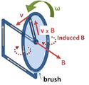
One can analyze examples like these by taking care that the path ∂Σ moves with the same velocity as the material.^[30] Alternatively, one can always correctly calculate the EMF by combining the Lorentz force law with the Maxwell–Faraday equation:^[17][31]

${\displaystyle {\mathcal {E}}=\int _{\partial \Sigma }(\mathbf {E} +\mathbf {v} _{m}\times \mathbf {B} )\cdot d\mathbf {l} =-\int _{\Sigma }{\frac {\partial \mathbf {B} }{\partial t}}\cdot d\mathbf {\Sigma } +\oint _{\partial \Sigma }(\mathbf {v} _{m}\times \mathbf {B} )\cdot d\mathbf {l} }$

where "it is very important to notice that (1) [v_m] is the velocity of the conductor ... not the velocity of the path element dl and (2) in general, the partial derivative with respect to time cannot be moved outside the integral since the area is a function of time".^[31]

Faraday's law and relativity

Two phenomena

Faraday's law is a single equation describing two different phenomena: the motional EMF generated by a magnetic force on a moving wire (see Lorentz force), and the transformer EMF generated by an electric force due to a changing magnetic field (due to the Maxwell–Faraday equation).

James Clerk Maxwell drew attention to this fact in his 1861 paper On Physical Lines of Force.^[32] In the latter half of Part II of that paper, Maxwell gives a separate physical explanation for each of the two phenomena.

A reference to these two aspects of electromagnetic induction is made in some modern textbooks.^[33] As Richard Feynman states:^[17]

So the "flux rule" that the emf in a circuit is equal to the rate of change of the magnetic flux through the circuit applies whether the flux changes because the field changes or because the circuit moves (or both) ...

Yet in our explanation of the rule we have used two completely distinct laws for the two cases – v × B for "circuit moves" and ∇ × E = −∂_tB for "field changes".

We know of no other place in physics where such a simple and accurate general principle requires for its real understanding an analysis in terms of two different phenomena.

— Richard P. Feynman, The Feynman Lectures on Physics

Einstein's view

Reflection on this apparent dichotomy was one of the principal paths that led Einstein to develop special relativity:

It is known that Maxwell's electrodynamics—as usually understood at the present time—when applied to moving bodies, leads to asymmetries which do not appear to be inherent in the phenomena. Take, for example, the reciprocal electrodynamic action of a magnet and a conductor.

The observable phenomenon here depends only on the relative motion of the conductor and the magnet, whereas the customary view draws a sharp distinction between the two cases in which either the one or the other of these bodies is in motion. For if the magnet is in motion and the conductor at rest, there arises in the neighbourhood of the magnet an electric field with a certain definite energy, producing a current at the places where parts of the conductor are situated.

But if the magnet is stationary and the conductor in motion, no electric field arises in the neighbourhood of the magnet. In the conductor, however, we find an electromotive force, to which in itself there is no corresponding energy, but which gives rise—assuming equality of relative motion in the two cases discussed—to electric currents of the same path and intensity as those produced by the electric forces in the former case.

Examples of this sort, together with unsuccessful attempts to discover any motion of the earth relative to the "light medium," suggest that the phenomena of electrodynamics as well as of mechanics possess no properties corresponding to the idea of absolute rest.

— Albert Einstein, On the Electrodynamics of Moving Bodies^[34]

Henry's law

From Wikipedia, the free encyclopedia

In chemistry, Henry's law is a gas law that states that the amount of dissolved gas is proportional to its partial pressure in the gas phase. The proportionality factor is called the Henry's law constant. It was formulated by the English chemist William Henry, who studied the topic in the early 19th century. In his publication about the quantity of gases absorbed by water,^[1] he described the results of his experiments:

..."water takes up, of gas condensed by one, two, or more additional atmospheres, a quantity which, ordinarily compressed, would be equal to twice, thrice, &c. the volume absorbed under the common pressure of the atmosphere."

An example where Henry's law is at play is in the depth-dependent dissolution of oxygen and nitrogen in the blood of underwater divers that changes during decompression, leading to decompression sickness. An everyday example is given by one's experience with carbonated soft drinks, which contain dissolved carbon dioxide. Before opening, the gas above the drink in its container is almost pure carbon dioxide, at a pressure higher than atmospheric pressure. After the bottle is opened, this gas escapes, moving the partial pressure of carbon dioxide above the liquid to be much lower, resulting in degassing as the dissolved carbon dioxide comes out of solution.

Fundamental types and variants of Henry's law constants

There are many ways to define the proportionality constant of Henry's law, which can be subdivided into two fundamental types: One possibility is to put the aqueous phase into the numerator and the gaseous phase into the denominator ("aq/gas").^[2] This results in the Henry's law solubility constant ${\displaystyle H}$. Its value increases with increased solubility. Alternatively, numerator and denominator can be switched ("gas/aq"), which results in the Henry's law volatility constant ${\displaystyle K_{\rm {H}}}$. The value of ${\displaystyle K_{\rm {H}}}$ decreases with increased solubility. There are several variants of both fundamental types. This results from the multiplicity of quantities that can be chosen to describe the composition of the two phases. Typical choices for the aqueous phase are molar concentration (${\displaystyle c_{\rm {a}}}$), molality (${\displaystyle b}$), and molar mixing ratio (${\displaystyle x}$). For the gas phase, molar concentration (${\displaystyle c_{\rm {g}}}$) and partial pressure (${\displaystyle p}$) are often used. It is not possible to use the gas-phase mixing ratio (${\displaystyle y}$) because at a given gas-phase mixing ratio, the aqueous-phase concentration ${\displaystyle c_{\rm {a}}}$ depends on the total pressure and thus the ratio ${\displaystyle y/c_{\rm {a}}}$ is not a constant.^[3] To specify the exact variant of the Henry's law constant, two superscripts are used. They refer to the numerator and the denominator of the definition. For example, ${\displaystyle H^{cp}}$ refers to the Henry solubility defined as ${\displaystyle c/p}$.

Henry's law solubility constants ${\displaystyle H}$

Henry solubility defined via concentration (${\displaystyle H^{cp}}$)

Atmospheric chemists often define the Henry solubility as

${\displaystyle H^{cp}=c_{\text{a}}/p}$.^[2]

Here ${\displaystyle c_{\text{a}}}$ is the concentration of a species in the aqueous phase, and ${\displaystyle p}$ is the partial pressure of that species in the gas phase under equilibrium conditions.^{[citation needed]}

The SI unit for ${\displaystyle H^{cp}}$ is mol/(m³ Pa); however, often the unit M/atm is used, since ${\displaystyle c_{\text{a}}}$ is usually expressed in M (1 M = 1 mol/dm³) and ${\displaystyle p}$ in atm (1 atm = 101325 Pa).^{[citation needed]}

The dimensionless Henry solubility ${\displaystyle H^{cc}}$

The Henry solubility can also be expressed as the dimensionless ratio between the aqueous-phase concentration ${\displaystyle c_{\text{a}}}$ of a species and its gas-phase concentration ${\displaystyle c_{\text{g}}}$:

${\displaystyle H^{cc}=c_{\text{a}}/c_{\text{g}}}$.^[2]

For an ideal gas, the conversion is:

${\displaystyle H^{cc}=H^{cp}\times RT}$ ,^[2]

where ${\displaystyle R}$ is the gas constant and ${\displaystyle T}$ is the temperature.

Sometimes, this dimensionless constant is called the "water-air partitioning coefficient" ${\displaystyle K_{\text{WA}}}$.^[4] It is closely related to the various, slightly different definitions of the "Ostwald coefficient" ${\displaystyle L}$, as discussed by Battino (1984).^[5]

Henry solubility defined via aqueous-phase mixing ratio (${\displaystyle H^{xp}}$)

Another Henry's law solubility constant is

${\displaystyle H^{xp}=x/p}$ .^[2]

Here ${\displaystyle x}$ is the molar mixing ratio in the aqueous phase. For a dilute aqueous solution the conversion between ${\displaystyle x}$ and ${\displaystyle c_{\text{a}}}$ is:

${\displaystyle c_{\text{a}}\approx x{\frac {\varrho _{\mathrm {H_{2}O} }}{M_{\mathrm {H_{2}O} }}}}$ ,^[2]

where ${\displaystyle \varrho _{\mathrm {H_{2}O} }}$ is the density of water and ${\displaystyle M_{\mathrm {H_{2}O} }}$ is the molar mass of water. Thus

${\displaystyle H^{xp}\approx {\frac {M_{\mathrm {H_{2}O} }}{\varrho _{\mathrm {H_{2}O} }}}\times H^{cp}}$ .^[2]

The SI unit for ${\displaystyle H^{xp}}$ is Pa⁻¹, although atm⁻¹ is still frequently used.^[2]

Henry solubility defined via molality (${\displaystyle H^{bp}}$)

It can be advantageous to describe the aqueous phase in terms of molality instead of concentration. The molality of a solution does not change with ${\displaystyle T}$, since it refers to the mass of the solvent. In contrast, the concentration ${\displaystyle c}$ does change with ${\displaystyle T}$, since the density of a solution and thus its volume are temperature-dependent. Defining the aqueous-phase composition via molality has the advantage that any temperature dependence of the Henry's law constant is a true solubility phenomenon and not introduced indirectly via a density change of the solution. Using molality, the Henry solubility can be defined as

${\displaystyle H^{bp}=b/p.}$

Here ${\displaystyle b}$ is used as the symbol for molality (instead of ${\displaystyle m}$) to avoid confusion with the symbol ${\displaystyle m}$ for mass. The SI unit for ${\displaystyle H^{bp}}$ is mol/(kg Pa). There is no simple way to calculate ${\displaystyle H^{cp}}$ from ${\displaystyle H^{bp}}$, since the conversion between concentration ${\displaystyle c_{\text{a}}}$ and molality ${\displaystyle b}$ involves all solutes of a solution. For a solution with a total of ${\displaystyle n}$ solutes with indices ${\displaystyle i=1,\ldots ,n}$, the conversion is:

${\displaystyle c_{\text{a}}={\frac {b\varrho }{1+\sum _{i=1}^{n}b_{i}M_{i}}},}$

where ${\displaystyle \varrho }$ is the density of the solution, and ${\displaystyle M_{i}}$ are the molar masses. Here ${\displaystyle b}$ is identical to one of the ${\displaystyle b_{i}}$ in the denominator. If there is only one solute, the equation simplifies to

${\displaystyle c_{\text{a}}={\frac {b\varrho }{1+bM}}.}$

Henry's law is only valid for dilute solutions where ${\displaystyle bM\ll 1}$ and ${\displaystyle \varrho \approx \varrho _{\mathrm {H_{2}O} }}$. In this case the conversion reduces further to

${\displaystyle c_{\text{a}}\approx b\varrho _{\mathrm {H_{2}O} },}$

and thus

${\displaystyle H^{bp}\approx H^{cp}/\varrho _{\mathrm {H_{2}O} }.}$

The Bunsen coefficient ${\displaystyle \alpha }$

According to Sazonov and Shaw, the dimensionless Bunsen coefficient ${\displaystyle \alpha }$ is defined as "the volume of saturating gas, V1, reduced to T° = 273.15 K, p° = 1 bar, which is absorbed by unit volume V₂* of pure solvent at the temperature of measurement and partial pressure of 1 bar."^[6] If the gas is ideal, the pressure cancels out, and the conversion to ${\displaystyle H^{cp}}$ is simply

${\displaystyle H^{cp}=\alpha \times {\frac {1}{RT^{\text{STP}}}}}$ ,

with ${\displaystyle T^{\text{STP}}}$ = 273.15 K. Note, that according to this definition, the conversion factor is not temperature-dependent.^{[citation needed]} Independent of the temperature that the Bunsen coefficient refers to, 273.15 K is always used for the conversion.^{[citation needed]} The Bunsen coefficient, which is named after Robert Bunsen, has been used mainly in the older literature.^{[citation needed]}

The Kuenen coefficient ${\displaystyle S}$

According to Sazonov and Shaw, the Kuenen coefficient ${\displaystyle S}$ is defined as "the volume of saturating gas V(g), reduced to T° = 273.15 K, p° = bar, which is dissolved by unit mass of pure solvent at the temperature of measurement and partial pressure 1 bar."^[6] If the gas is ideal, the relation to ${\displaystyle H^{cp}}$ is

${\displaystyle H^{cp}=S\times {\frac {\varrho }{RT^{\text{STP}}}}}$ ,^{[citation needed][original research?]}

where ${\displaystyle \varrho }$ is the density of the solvent, and ${\displaystyle T^{\text{STP}}}$ = 273.15 K. The SI unit for ${\displaystyle S}$ is m³/kg.^[6] The Kuenen coefficient, which is named after Johannes Kuenen, has been used mainly in the older literature, and IUPAC considers it to be obsolete.^[7]

Henry's law volatility constants ${\displaystyle K_{\text{H}}}$

The Henry volatility defined via concentration (${\displaystyle K_{\text{H}}^{pc}}$)

A common way to define a Henry volatility is dividing the partial pressure by the aqueous-phase concentration:

${\displaystyle K_{\text{H}}^{pc}=p/c_{\text{a}}=1/H^{cp}.}$

The SI unit for ${\displaystyle K_{\text{H}}^{pc}}$ is Pa m³/mol.

The Henry volatility defined via aqueous-phase mixing ratio (${\displaystyle K_{\text{H}}^{px}}$)

Another Henry volatility is

${\displaystyle K_{\text{H}}^{px}=p/x=1/H^{xp}.}$

The SI unit for ${\displaystyle K_{\text{H}}^{px}}$ is Pa. However, atm is still frequently used.

The dimensionless Henry volatility ${\displaystyle K_{\text{H}}^{cc}}$

The Henry volatility can also be expressed as the dimensionless ratio between the gas-phase concentration ${\displaystyle c_{\text{g}}}$ of a species and its aqueous-phase concentration ${\displaystyle c_{\text{a}}}$:

${\displaystyle K_{\text{H}}^{cc}=c_{\text{g}}/c_{\text{a}}=1/H^{cc}.}$

In chemical engineering and environmental chemistry, this dimensionless constant is often called the air–water partitioning coefficient ${\displaystyle K_{\text{AW}}}$.

Values of Henry's law constants

A large compilation of Henry's law constants has been published by Sander (2015).^[2] A few selected values are shown in the table below:

Henry's law constants (gases in water at 298.15 K)

equation:	${\displaystyle K_{\text{H}}^{pc}={\frac {p}{c_{\text{aq}}}}}$	${\displaystyle H^{cp}={\frac {c_{\text{aq}}}{p}}}$	${\displaystyle K_{\text{H}}^{px}={\frac {p}{x}}}$	${\displaystyle H^{cc}={\frac {c_{\text{aq}}}{c_{\text{gas}}}}}$
unit:	${\displaystyle {\frac {{\text{L}}\cdot {\text{atm}}}{\text{mol}}}}$	${\displaystyle {\frac {\text{mol}}{{\text{L}}\cdot {\text{atm}}}}}$	${\displaystyle {\text{atm}}}$	(dimensionless)
O2	770	1.3×10−3	4.3×104	3.2×10−2
H2	1300	7.8×10−4	7.1×104	1.9×10−2
CO2	29	3.4×10−2	1.6×103	8.3×10−1
N2	1600	6.1×10−4	9.1×104	1.5×10−2
He	2700	3.7×10−4	1.5×105	9.1×10−3
Ne	2200	4.5×10−4	1.2×105	1.1×10−2
Ar	710	1.4×10−3	4.0×104	3.4×10−2
CO	1100	9.5×10−4	5.8×104	2.3×10−2

Temperature dependence

When the temperature of a system changes, the Henry constant also changes. The temperature dependence of equilibrium constants can generally be described with the van 't Hoff equation, which also applies to Henry's law constants:

${\displaystyle {\frac {\mathrm {d} \ln H}{\mathrm {d} (1/T)}}={\frac {-\Delta _{\text{sol}}H}{R}},}$

where ${\displaystyle \Delta _{\text{sol}}H}$ is the enthalpy of dissolution. Note that the letter ${\displaystyle H}$ in the symbol ${\displaystyle \Delta _{\text{sol}}H}$ refers to enthalpy and is not related to the letter ${\displaystyle H}$ for Henry's law constants. Integrating the above equation and creating an expression based on ${\displaystyle H^{\circ }}$ at the reference temperature ${\displaystyle T^{\circ }}$ = 298.15 K yields:

${\displaystyle H(T)=H^{\circ }\times \exp \displaystyle \left[{\frac {-\Delta _{\text{sol}}H}{R}}\left({\frac {1}{T}}-{\frac {1}{T^{\circ }}}\right)\right].}$

The van 't Hoff equation in this form is only valid for a limited temperature range in which ${\displaystyle \Delta _{\text{sol}}H}$ does not change much with temperature.

The following table lists some temperature dependencies:

Values of ${\displaystyle -\Delta _{\text{sol}}H/R}$ (in K)

O2	H2	CO2	N2	He	Ne	Ar	CO
1700	500	2400	1300	230	490	1300	1300

Solubility of permanent gases usually decreases with increasing temperature at around room temperature. However, for aqueous solutions, the Henry's law solubility constant for many species goes through a minimum. For most permanent gases, the minimum is below 120 °C. Often, the smaller the gas molecule (and the lower the gas solubility in water), the lower the temperature of the maximum of the Henry's law constant. Thus, the maximum is at about 30 °C for helium, 92 to 93 °C for argon, nitrogen and oxygen, and 114 °C for xenon.^[8]

Effective Henry's law constants H_eff

The Henry's law constants mentioned so far do not consider any chemical equilibria in the aqueous phase. This type is called the "intrinsic" (or "physical") Henry's law constant. For example, the intrinsic Henry's law solubility constant of formaldehyde can be defined as

${\displaystyle H^{{\ce {cp}}}={\frac {c({\ce {H2CO}})}{p({\ce {H2CO}})}}.}$

In aqueous solution, methanal is almost completely hydrated:

${\displaystyle {\ce {{H2CO}+ {H2O}<=> {H2C(OH)2}}}}$

The total concentration of dissolved methanal is

${\displaystyle c_{{\ce {tot}}}=c({\ce {H2CO}})+c({\ce {H2C(OH)2}}).}$

Taking this equilibrium into account, an effective Henry's law constant ${\displaystyle H_{{\ce {eff}}}}$ can be defined as

${\displaystyle H_{{\ce {eff}}}={\frac {c_{{\ce {tot}}}}{p({\ce {H2CO}})}}={\frac {c({\ce {H2CO}})+c({\ce {H2C(OH)2}})}{p({\ce {H2CO}})}}.}$

For acids and bases, the effective Henry's law constant is not a useful quantity because it depends on the pH of the solution.^{[verification needed]} In order to obtain a pH-independent constant, the product of the intrinsic Henry's law constant ${\displaystyle H^{{\ce {cp}}}}$ and the acidity constant ${\displaystyle K_{{\ce {A}}}}$ is often used for strong acids like hydrochloric acid (HCl):

${\displaystyle H'=H^{{\ce {cp}}}\times K_{{\ce {A}}}={\frac {c({\ce {H+}})\times c({\ce {Cl^-}})}{p({\ce {HCl}})}}.}$

Although ${\displaystyle H'}$ is usually also called a Henry's law constant, it should be noted that it is a different quantity and it has different units than ${\displaystyle H^{{\ce {cp}}}}$.

Dependence on ionic strength (Sechenov equation)

Values of Henry's law constants for aqueous solutions depend on the composition of the solution, i.e., on its ionic strength and on dissolved organics. In general, the solubility of a gas decreases with increasing salinity ("salting out"). However, a "salting in" effect has also been observed, for example for the effective Henry's law constant of glyoxal. The effect can be described with the Sechenov equation, named after the Russian physiologist Ivan Sechenov (sometimes the German transliteration "Setschenow" of the Cyrillic name Се́ченов is used). There are many alternative ways to define the Sechenov equation, depending on how the aqueous-phase composition is described (based on concentration, molality, or molar fraction) and which variant of the Henry's law constant is used. Describing the solution in terms of molality is preferred because molality is invariant to temperature and to the addition of dry salt to the solution. Thus, the Sechenov equation can be written as

${\displaystyle \log \left({\frac {H_{0}^{bp}}{H^{bp}}}\right)=k_{\text{s}}\times b({\text{salt}}),}$

where ${\displaystyle H_{0}^{bp}}$ is the Henry's law constant in pure water, ${\displaystyle H^{bp}}$ is the Henry's law constant in the salt solution, ${\displaystyle k_{\text{s}}}$ is the molality-based Sechenov constant, and ${\displaystyle b({\text{salt}})}$ is the molality of the salt.

Non-ideal solutions

Henry's law has been shown to apply to a wide range of solutes in the limit of "infinite dilution" (x → 0), including non-volatile substances such as sucrose. In these cases, it is necessary to state the law in terms of chemical potentials. For a solute in an ideal dilute solution, the chemical potential depends only on the concentration. For non-ideal solutions, the activity coefficients of the components must be taken into account:

${\displaystyle \mu =\mu _{c}^{\circ }+RT\ln {\frac {\gamma _{c}c}{c^{\circ }}}}$,

where ${\displaystyle \gamma _{c}={\frac {K_{{\text{H}},c}}{p^{*}}}}$ for a volatile solute; c° = 1 mol/L.

For non-ideal solutions, the activity coefficient γ_c depends on the concentration and must be determined at the concentration of interest. The activity coefficient can also be obtained for non-volatile solutes, where the vapor pressure of the pure substance is negligible, by using the Gibbs-Duhem relation:

${\displaystyle \sum _{i}n_{i}d\mu _{i}=0.}$

By measuring the change in vapor pressure (and hence chemical potential) of the solvent, the chemical potential of the solute can be deduced.

The standard state for a dilute solution is also defined in terms of infinite-dilution behavior. Although the standard concentration c° is taken to be 1 mol/l by convention, the standard state is a hypothetical solution of 1 mol/l in which the solute has its limiting infinite-dilution properties. This has the effect that all non-ideal behavior is described by the activity coefficient: the activity coefficient at 1 mol/l is not necessarily unity (and is frequently quite different from unity).

All the relations above can also be expressed in terms of molalities b rather than concentrations, e.g.:

${\displaystyle \mu =\mu _{b}^{\circ }+RT\ln {\frac {\gamma _{b}b}{b^{\circ }}},}$

where ${\displaystyle \gamma _{b}={\frac {K_{{\text{H}},b}}{p^{*}}}}$ for a volatile solute; b° = 1 mol/kg.

The standard chemical potential μ_m°, the activity coefficient γ_m and the Henry's law constant K_H,b all have different numerical values when molalities are used in place of concentrations.

Solvent mixtures

Henry law constant H_{2, M} for a gas 2 in a mixture of solvents 1 and 3 is related to the constants for individual solvents H₂₁ and H₂₃:

${\displaystyle \ln H_{2M}=x_{1}\ln H_{21}+x_{2}\ln H_{23}-a_{13}x_{1}x_{3}}$

where a₁₃ is the interaction parameter of the solvents from Wohl expansion of the excess chemical potential of the ternary mixtures.

Miscellaneous

In geochemistry

In geochemistry, a version of Henry's law applies to the solubility of a noble gas in contact with silicate melt. One equation used is

${\displaystyle C_{\text{melt}}/C_{\text{gas}}=\exp \left[-\beta (\mu _{\text{melt}}^{\text{E}}-\mu _{\text{gas}}^{\text{E}})\right],}$

where

C is the number concentrations of the solute gas in the melt and gas phases,

β = 1/k_BT, an inverse temperature parameter (k_B is the Boltzmann constant),

µ^E is the excess chemical potentials of the solute gas in the two phases.

Comparison to Raoult's law

Henry's law is a limiting law that only applies for "sufficiently dilute" solutions. The range of concentrations in which it applies becomes narrower the more the system diverges from ideal behavior. Roughly speaking, that is the more chemically "different" the solute is from the solvent.

For a dilute solution, the concentration of the solute is approximately proportional to its mole fraction x, and Henry's law can be written as

${\displaystyle p=K_{\text{H}}x.}$

This can be compared with Raoult's law:

${\displaystyle p=p^{*}x,}$

where p* is the vapor pressure of the pure component.

At first sight, Raoult's law appears to be a special case of Henry's law, where K_H = p*. This is true for pairs of closely related substances, such as benzene and toluene, which obey Raoult's law over the entire composition range: such mixtures are called "ideal mixtures".

The general case is that both laws are limit laws, and they apply at opposite ends of the composition range. The vapor pressure of the component in large excess, such as the solvent for a dilute solution, is proportional to its mole fraction, and the constant of proportionality is the vapor pressure of the pure substance (Raoult's law). The vapor pressure of the solute is also proportional to the solute's mole fraction, but the constant of proportionality is different and must be determined experimentally (Henry's law). In mathematical terms:

Raoult's law: ${\displaystyle \lim _{x\to 1}\left({\frac {p}{x}}\right)=p^{*}.}$

Henry's law: ${\displaystyle \lim _{x\to 0}\left({\frac {p}{x}}\right)=K_{\text{H}}.}$

Raoult's law can also be related to non-gas solutes.