From Wikipedia, the free encyclopedia

Some trajectories of a harmonic oscillator according to Newton's laws of classical mechanics (A–B), and according to the Schrödinger equation of quantum mechanics (C–H). In A–B, the particle (represented as a ball attached to a spring) oscillates back and forth. In C–H, some solutions to the Schrödinger Equation are shown, where the horizontal axis is position, and the vertical axis is the real part (blue) or imaginary part (red) of the wavefunction. C, D, E, F, but not G, H, are energy eigenstates. H is a coherent state—a quantum state that approximates the classical trajectory.
The quantum harmonic oscillator is the quantum-mechanical analog of the classical harmonic oscillator. Because an arbitrary potential can usually be approximated as a harmonic potential at the vicinity of a stable equilibrium point, it is one of the most important model systems in quantum mechanics. Furthermore, it is one of the few quantum-mechanical systems for which an exact, analytical solution is known.[1][2][3]
One-dimensional harmonic oscillator
Hamiltonian and energy eigenstates


One may write the time-independent Schrödinger equation,

One may solve the differential equation representing this eigenvalue problem in the coordinate basis, for the wave function ⟨x|ψ⟩ = ψ(x), using a spectral method. It turns out that there is a family of solutions. In this basis, they amount to


Note that the ground state probability density is concentrated at the origin. This means the particle spends most of its time at the bottom of the potential well, as we would expect for a state with little energy. As the energy increases, the probability density becomes concentrated at the classical "turning points", where the state's energy coincides with the potential energy. This is consistent with the classical harmonic oscillator, in which the particle spends most of its time (and is therefore most likely to be found) at the turning points, where it is the slowest. The correspondence principle is thus satisfied. Moreover, special nondispersive wave packets, with minimum uncertainty, called coherent states in fact oscillate very much like classical objects, as illustrated in the figure; they are not eigenstates of the Hamiltonian.
Ladder operator method

The spectral method solution, though straightforward, is rather tedious. The "ladder operator" method, developed by Paul Dirac, allows us to extract the energy eigenvalues without directly solving the differential equation. Furthermore, it is readily generalizable to more complicated problems, notably in quantum field theory. Following this approach, we define the operators a and its adjoint a†,


From the relations above, we can also define a number operator N, which has the following property:


![[a,a^{\dagger}]=1,\qquad[N,a^{\dagger}]=a^{\dagger},\qquad[N,a]=-a,](http://upload.wikimedia.org/math/8/3/5/835fa687285d040f2814adba5f31078a.png)

The commutation property yields
![\begin{align}
Na^{\dagger}|n\rangle&=\left(a^{\dagger}N+[N,a^{\dagger}]\right)|n\rangle\\&=\left(a^{\dagger}N+a^{\dagger}\right)|n\rangle\\&=(n+1)a^{\dagger}|n\rangle,
\end{align}](http://upload.wikimedia.org/math/4/e/0/4e019146a7b00031bbc0f206d6bc4f7d.png)

For this reason, a is called a "lowering operator", and a† a "raising operator". The two operators together are called ladder operators. In quantum field theory, a and a† are alternatively called "annihilation" and "creation" operators because they destroy and create particles, which correspond to our quanta of energy.
Given any energy eigenstate, we can act on it with the lowering operator, a, to produce another eigenstate with ħω less energy. By repeated application of the lowering operator, it seems that we can produce energy eigenstates down to E = −∞. However, since


Arbitrary eigenstates can be expressed in terms of |0⟩,

- Proof:

![\begin{align}
\langle n\mid aa^\dagger |n\rangle&=\langle n|\left([a,a^\dagger]+a^\dagger a\right)\mid n \rangle = \langle n|(N+1)|n\rangle=n+1\\\Rightarrow a^\dagger \mid n\rangle & =\sqrt{n+1}\mid n+1\rangle \\ \Rightarrow|n\rangle&=\frac{a^\dagger}{\sqrt{n}} \mid n-1\rangle=\frac{(a^\dagger)^2}{\sqrt{n(n-1)}}\mid n-2\rangle = \cdots = \frac{(a^\dagger)^{n}}{\sqrt{n!}}|0\rangle.
\end{align}](http://upload.wikimedia.org/math/2/a/a/2aaa469bf29e33a723581a86d48d9a1d.png)


Natural length and energy scales
The quantum harmonic oscillator possesses natural scales for length and energy, which can be used to simplify the problem. These can be found by nondimensionalization.The result is that, if we measure energy in units of ħω and distance in units of √ħ/(mω), then the Hamiltonian simplifies to


To avoid confusion, we will not adopt these "natural units" in this article. However, they frequently come in handy when performing calculations, by bypassing clutter.
For example, the fundamental solution (propagator) of H−i∂t, the time-dependent Schroedinger operator for this oscillator, simply boils down to the Mehler kernel,[4][5]


Phase space solutions
In the phase space formulation of quantum mechanics, solutions to the quantum harmonic oscillator in several different representations of the quasiprobability distribution can be written in closed form. The most widely used of these is for the Wigner quasiprobability distribution, which has the solution

This example illustrates how the Hermite and Laguerre polynomials are linked through the Wigner map.
N-dimensional harmonic oscillator
The one-dimensional harmonic oscillator is readily generalizable to N dimensions, where N = 1, 2, 3, ... . In one dimension, the position of the particle was specified by a single coordinate, x. In N dimensions, this is replaced by N position coordinates, which we label x1, ..., xN. Corresponding to each position coordinate is a momentum; we label these p1, ..., pN. The canonical commutation relations between these operators are![\begin{align}
{[}x_i , p_j{]} &= i\hbar\delta_{i,j} \\
{[}x_i , x_j{]} &= 0 \\
{[}p_i , p_j{]} &= 0
\end{align}](http://upload.wikimedia.org/math/c/8/8/c88881718d6df249ffbea5cf03e247c9.png)

 potential, which allows the potential energy to be separated into terms depending on one coordinate each.
This observation makes the solution straightforward. For a particular set of quantum numbers {n} the energy eigenfunctions for the N-dimensional oscillator are expressed in terms of the 1-dimensional eigenfunctions as:


 is an element in the defining matrix representation of U(N).
The energy levels of the system are
![E = \hbar \omega \left[(n_1 + \cdots + n_N) + {N\over 2}\right].](http://upload.wikimedia.org/math/3/4/3/3430388d7bcecc60401524afbadddfea.png)

The degeneracy can be calculated relatively easily. As an example, consider the 3-dimensional case: Define n = n1 + n2 + n3. All states with the same n will have the same energy. For a given n, we choose a particular n1. Then n2 + n3 = n − n1. There are n − n1 + 1 possible pairs {n2, n3}. n2 can take on the values 0 to n − n1, and for each n2 the value of n3 is fixed. The degree of degeneracy therefore is:


 and
and  , which are the same constraints as in integer partition.
Example: 3D isotropic harmonic oscillator
The Schrödinger equation of a spherically-symmetric three-dimensional harmonic oscillator can be solved explicitly by separation of variables; see this article for the present case. This procedure is analogous to the separation performed in the hydrogen-like atom problem, but with the spherically symmetric potential
The solution reads

 is a normalization constant;
  ;
;
 is a normalization constant;
  ;
;
 is a spherical harmonic function;
- ħ is the reduced Planck constant:

 is a
is a 


Harmonic oscillators lattice: phonons
We can extend the notion of a harmonic oscillator to a one lattice of many particles. Consider a one-dimensional quantum mechanical harmonic chain of N identical atoms. This is the simplest quantum mechanical model of a lattice, and we will see how phonons arise from it. The formalism that we will develop for this model is readily generalizable to two and three dimensions.As in the previous section, we denote the positions of the masses by x1,x2,..., as measured from their equilibrium positions (i.e. xi = 0 if the particle i is at its equilibrium position.) In two or more dimensions, the xi are vector quantities. The Hamiltonian for this system is

We introduce, then, a set of N "normal coordinates" Qk, defined as the discrete Fourier transforms of the xs, and N "conjugate momenta" Π defined as the Fourier transforms of the ps,


This preserves the desired commutation relations in either real space or wave vector space
![\begin{align}
\left[x_l , p_m \right]&=i\hbar\delta_{l,m} \\
\left[ Q_k , \Pi_{k'} \right] &={1\over N} \sum_{l,m} e^{ikal} e^{-ik'am} [x_l , p_m ] \\
&= {i \hbar\over N} \sum_{m} e^{iam(k-k')} = i\hbar\delta_{k,k'} \\
\left[ Q_k , Q_{k'} \right] &= \left[ \Pi_k , \Pi_{k'} \right] = 0 ~.
\end{align}](http://upload.wikimedia.org/math/3/9/0/390f76ea3d2fa7642d59adb9411852d9.png)


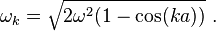

The form of the quantization depends on the choice of boundary conditions; for simplicity, we impose periodic boundary conditions, defining the (N + 1)th atom as equivalent to the first atom. Physically, this corresponds to joining the chain at its ends. The resulting quantization is

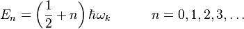
The harmonic oscillator eigenvalues or energy levels for the mode ωk are
All quantum systems show wave-like and particle-like properties. The particle-like properties of the phonon are best understood using the methods of second quantization and operator techniques described later.[6]
Applications
- The vibrations of a diatomic molecule are an example of a two-body version of the quantum harmonic oscillator. In this case, the angular frequency is given by
-
- where μ = m1m2/(m1 + m2) is the reduced mass and is determined by the masses m1, m2 of the two atoms.[7]

- The Hooke's atom is a simple model of the helium atom using the quantum harmonic oscillator
- Modelling phonons, as discussed above
- A charge, q, with mass, m, in a uniform magnetic field, B, is an example of a one-dimensional quantum harmonic oscillator: the Landau quantization.


