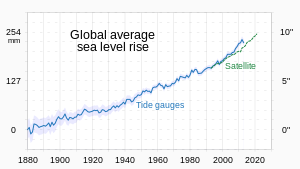
Between 1901 and 2018, average global sea level rose by 15–25 cm (6–10 in), an average of 1–2 mm (0.039–0.079 in) per year. This rate accelerated to 4.62 mm (0.182 in)/yr for the decade 2013–2022. Climate change due to human activities is the main cause. Between 1993 and 2018, thermal expansion of water accounted for 42% of sea level rise. Melting temperate glaciers accounted for 21%, while polar glaciers in Greenland accounted for 15% and those in Antarctica for 8%.
Sea level rise lags behind changes in the Earth's temperature, and sea level rise will therefore continue to accelerate between now and 2050 in response to warming that has already happened. What happens after that depends on human greenhouse gas emissions. Sea level rise would slow down between 2050 and 2100 if there are very deep cuts in emissions. It could then reach slightly over 30 cm (1 ft) from now by 2100. With high emissions it would accelerate. It could rise by 1.01 m (3+1⁄3 ft) or even 1.6 m (5+1⁄3 ft) by then. In the long run, sea level rise would amount to 2–3 m (7–10 ft) over the next 2000 years if warming amounts to 1.5 °C (2.7 °F). It would be 19–22 metres (62–72 ft) if warming peaks at 5 °C (9.0 °F).
Rising seas affect every coastal and island population on Earth. This can be through flooding, higher storm surges, king tides, and tsunamis. There are many knock-on effects. They lead to loss of coastal ecosystems like mangroves. Crop yields may reduce because of increasing salt levels in irrigation water. Damage to ports disrupts sea trade. The sea level rise projected by 2050 will expose places currently inhabited by tens of millions of people to annual flooding. Without a sharp reduction in greenhouse gas emissions, this may increase to hundreds of millions in the latter decades of the century. Areas not directly exposed to rising sea levels could be vulnerable to large-scale migration and economic disruption.
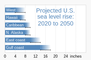
Local factors like tidal range or land subsidence will greatly affect the severity of impacts. There is also the varying resilience and adaptive capacity of ecosystems and countries which will result in more or less pronounced impacts. For instance, sea level rise in the United States (particularly along the US East Coast) is likely to be 2 to 3 times greater than the global average by the end of the century. Yet, of the 20 countries with the greatest exposure to sea level rise, 12 are in Asia, including Indonesia, Bangladesh and the Philippines. The greatest impact on human populations in the near term will occur in the low-lying Caribbean and Pacific islands. Sea level rise will make many of them uninhabitable later this century.
Societies can adapt to sea level rise in multiple ways. Managed retreat, accommodating coastal change, or protecting against sea level rise through hard-construction practices like seawalls are hard approaches. There are also soft approaches such as dune rehabilitation and beach nourishment. Sometimes these adaptation strategies go hand in hand. At other times choices must be made among different strategies. A managed retreat strategy is difficult if an area's population is increasing rapidly. This is a particularly acute problem for Africa. Poorer nations may also struggle to implement the same approaches to adapt to sea level rise as richer states. Sea level rise at some locations may be compounded by other environmental issues. One example is subsidence in sinking cities. Coastal ecosystems typically adapt to rising sea levels by moving inland. Natural or artificial barriers may make that impossible.
Observations
Between 1901 and 2018, the global mean sea level rose by about 20 cm (7.9 in). More precise data gathered from satellite radar measurements found a rise of 7.5 cm (3.0 in) from 1993 to 2017 (average of 2.9 mm (0.11 in)/yr). This accelerated to 4.62 mm (0.182 in)/yr for 2013–2022.
Regional variations
Sea level rise is not uniform around the globe. Some land masses are moving up or down as a consequence of subsidence (land sinking or settling) or post-glacial rebound (land rising as melting ice reduces weight). Therefore, local relative sea level rise may be higher or lower than the global average. Changing ice masses also affect the distribution of sea water around the globe through gravity.
When a glacier or ice sheet melts, it loses mass. This reduces its gravitational pull. In some places near current and former glaciers and ice sheets, this has caused water levels to drop. At the same time water levels will increase more than average further away from the ice sheet. Thus ice loss in Greenland affects regional sea level differently than the equivalent loss in Antarctica. On the other hand, the Atlantic is warming at a faster pace than the Pacific. This has consequences for Europe and the U.S. East Coast. The East Coast sea level is rising at 3–4 times the global average. Scientists have linked extreme regional sea level rise on the US Northeast Coast to the downturn of the Atlantic meridional overturning circulation (AMOC).
Many ports, urban conglomerations, and agricultural regions stand on river deltas. Here land subsidence contributes to much higher relative sea level rise. Unsustainable extraction of groundwater and oil and gas is one cause. Levees and other flood management practices are another. They prevent sediments from accumulating. These would otherwise compensate for the natural settling of deltaic soils. Estimates for total human-caused subsidence in the Rhine-Meuse-Scheldt delta (Netherlands) are 3–4 m (10–13 ft), over 3 m (10 ft) in urban areas of the Mississippi River Delta (New Orleans), and over 9 m (30 ft) in the Sacramento–San Joaquin River Delta. On the other hand, relative sea level around the Hudson Bay in Canada and the northern Baltic is falling due to post-glacial isostatic rebound.
Projections
There are two complementary ways to model sea level rise (SLR) and project the future. The first uses process-based modeling. This combines all relevant and well-understood physical processes in a global physical model. This approach calculates the contributions of ice sheets with an ice-sheet model and computes rising sea temperature and expansion with a general circulation model. The processes are imperfectly understood, but this approach has the advantage of predicting non-linearities and long delays in the response, which studies of the recent past will miss.
The other approach employs semi-empirical techniques. These use historical geological data to determine likely sea level responses to a warming world, and some basic physical modeling. These semi-empirical sea level models rely on statistical techniques. They use relationships between observed past contributions to global mean sea level and temperature. Scientists developed this type of modeling because most physical models in previous Intergovernmental Panel on Climate Change (IPCC) literature assessments had underestimated the amount of sea level rise compared to 20th century observations.
Projections for the 21st century

Intergovernmental Panel on Climate Change is the largest and most influential scientific organization on climate change, and since 1990, it provides several plausible scenarios of 21st century sea level rise in each of its major reports. The differences between scenarios are mainly due to uncertainty about future greenhouse gas emissions. These depend on future economic developments, and also future political action which is hard to predict. Each scenario provides an estimate for sea level rise as a range with a lower and upper limit to reflect the unknowns. The scenarios in the 2013-2014 Fifth Assessment Report (AR5) were called Representative Concentration Pathways, or RCPs and the scenarios in the IPCC Sixth Assessment Report (AR6) are known as Shared Socioeconomic Pathways, or SSPs. A large difference between the two was the addition of SSP1-1.9 to AR6, which represents meeting the best Paris climate agreement goal of 1.5 °C (2.7 °F). In that case, the likely range of sea level rise by 2100 is 28–55 cm (11–21+1⁄2 in).
The lowest scenario in AR5, RCP2.6, would see greenhouse gas emissions low enough to meet the goal of limiting warming by 2100 to 2 °C (3.6 °F). It shows sea level rise in 2100 of about 44 cm (17 in) with a range of 28–61 cm (11–24 in). The "moderate" scenario, where CO2 emissions take a decade or two to peak and its atmospheric concentration does not plateau until 2070s is called RCP 4.5. Its likely range of sea level rise is 36–71 cm (14–28 in). The highest scenario in RCP8.5 pathway sea level would rise between 52 and 98 cm (20+1⁄2 and 38+1⁄2 in). AR6 had equivalents for both scenarios, but it estimated larger sea level rise under both. In AR6, the SSP1-2.6 pathway results in a range of 32–62 cm (12+1⁄2–24+1⁄2 in) by 2100. The "moderate" SSP2-4.5 results in a 44–76 cm (17+1⁄2–30 in) range by 2100 and SSP5-8.5 led to 65–101 cm (25+1⁄2–40 in).
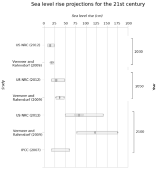
Further, AR5 was criticized by multiple researchers for excluding detailed estimates the impact of "low-confidence" processes like marine ice sheet and marine ice cliff instability, which can substantially accelerate ice loss to potentially add "tens of centimeters" to sea level rise within this century. AR6 includes a version of SSP5-8.5 where these processes take place, and in that case, sea level rise of up to 1.6 m (5+1⁄3 ft) by 2100 could not be ruled out. The general increase of projections in AR6 was caused by the observed ice-sheet erosion in Greenland and Antarctica matching the upper-end range of the AR5 projections by 2020, and the finding that AR5 projections were likely too slow next to an extrapolation of observed sea level rise trends, while the subsequent reports had improved in this regard.
Notably, some scientists believe that ice sheet processes may accelerate sea level rise even at temperatures below the highest possible scenario, though not as much. For instance, a 2017 study from the University of Melbourne researchers suggested that these processes increase RCP2.6 sea level rise by about one quarter, RCP4.5 sea level rise by one half and practically double RCP8.5 sea level rise. A 2016 study led by Jim Hansen hypothesized that vulnerable ice sheet section collapse can lead to near-term exponential sea level rise acceleration, with a doubling time of 10, 20, or 40 years. Such acceleration would lead to multi-meter sea level rise in 50, 100, or 200 years, respectively, but it remains a minority view amongst the scientific community.
For comparison, a major scientific survey of 106 experts in 2020 found that even when accounting for instability processes they had estimated a median sea level rise of 45 cm (17+1⁄2 in) by 2100 for RCP2.6, with a 5%-95% range of 21–82 cm (8+1⁄2–32+1⁄2 in). For RCP8.5, the experts estimated a median of 93 cm (36+1⁄2 in) by 2100 and a 5%-95% range of 45–165 cm (17+1⁄2–65 in). Similarly, NOAA in 2022 had suggested that there is a 50% probability of 0.5 m (19+1⁄2 in) sea level rise by 2100 under 2 °C (3.6 °F), which increases to >80% to >99% under 3–5 °C (5.4–9.0 °F). Year 2019 elicitation of 22 ice sheet experts suggested a median SLR of 30 cm (12 in) by 2050 and 70 cm (27+1⁄2 in) by 2100 in the low emission scenario and the median of 34 cm (13+1⁄2 in) by 2050 and 110 cm (43+1⁄2 in) by 2100 in a high emission scenario. They also estimated a small chance of sea levels exceeding 1 meter by 2100 even in the low emission scenario and of going beyond 2 metres in the high emission scenario, with the latter causing the displacement of 187 million people.
Post-2100 sea level rise


Even if the temperature stabilizes, significant sea-level rise (SLR) will continue for centuries, consistent with paleo records of sea level rise. This is due to the high level of inertia in the carbon cycle and the climate system, owing to factors such as the slow diffusion of heat into the deep ocean, leading to a longer climate response time. After 500 years, sea level rise from thermal expansion alone may have reached only half of its eventual level. Models suggest this may lie within ranges of 0.5–2 m (1+1⁄2–6+1⁄2 ft). Additionally, tipping points of Greenland and Antarctica ice sheets are likely to play a larger role over such timescales. Ice loss from Antarctica is likely to dominate very long-term SLR, especially if the warming exceeds 2 °C (3.6 °F). Continued carbon dioxide emissions from fossil fuel sources could cause additional tens of metres of sea level rise, over the next millennia. The available fossil fuel on Earth is enough to melt the entire Antarctic ice sheet, causing about 58 m (190 ft) of sea level rise.
Based on research into multimillennial sea level rise, AR6 was able to create medium agreement estimates for the amount of sea level rise over the next 2,000 years, depending on the peak of global warming, which project that:
- At a warming peak of 1.5 °C (2.7 °F), global sea levels would rise 2–3 m (6+1⁄2–10 ft)
- At a warming peak of 2 °C (3.6 °F), sea levels would rise 2–6 m (6+1⁄2–19+1⁄2 ft)
- At a warming peak of 5 °C (9.0 °F), sea levels would rise 19–22 m (62+1⁄2–72 ft)
Sea levels would continue to rise for several thousand years after the ceasing of emissions, due to the slow nature of climate response to heat. The same estimates on a timescale of 10,000 years project that:
- At a warming peak of 1.5 °C (2.7 °F), global sea levels would rise 6–7 m (19+1⁄2–23 ft)
- At a warming peak of 2 °C (3.6 °F), sea levels would rise 8–13 m (26–42+1⁄2 ft)
- At a warming peak of 5 °C (9.0 °F), sea levels would rise 28–37 m (92–121+1⁄2 ft)
With better models and observational records, several studies have attempted to project SLR for the centuries immediately after 2100. This remains largely speculative. An April 2019 expert elicitation asked 22 experts about total sea level rise projections for the years 2200 and 2300 under its high, 5 °C warming scenario. It ended up with 90% confidence intervals of −10 cm (4 in) to 740 cm (24+1⁄2 ft) and −9 cm (3+1⁄2 in) to 970 cm (32 ft), respectively. Negative values represent the extremely low probability of very large increases in the ice sheet surface mass balance due to climate change-induced increase in precipitation. An elicitation of 106 experts led by Stefan Rahmstorf also included 2300 for RCP2.6 and RCP8.5. The former had the median of 118 cm (46+1⁄2 in), and a 5%-95% range of 24–311 cm (9+1⁄2–122+1⁄2 in). The latter had the median of 329 cm (129+1⁄2 in), and a 5%-95% range of 88–783 cm (34+1⁄2–308+1⁄2 in).
By 2021, AR6 was also able to provide estimates for sea level rise in 2150 alongside the 2100 estimates for the first time. This showed that keeping warming at 1.5 °C under the SSP1-1.9 scenario would result in sea level rise in the 17-83% range of 37–86 cm (14+1⁄2–34 in). In the SSP1-2.6 pathway the range would be 46–99 cm (18–39 in), for SSP2-4.5 a 66–133 cm (26–52+1⁄2 in) range by 2100 and for SSP5-8.5 a rise of 98–188 cm (38+1⁄2–74 in). It stated that the "low-confidence, high impact" projected 0.63–1.60 m (2–5 ft) mean sea level rise by 2100, and that by 2150, the total sea level rise in his scenario would be in the range of 0.98–4.82 m (3–16 ft) by 2150. AR6 also provided lower-confidence estimates for year 2300 sea level rise under SSP1-2.6 and SSP5-8.5 with various impact assumptions. In the best case scenario, under SSP1-2.6 with no ice sheet acceleration after 2100, the estimate was only 0.8–2.0 metres (2.6–6.6 ft). In the worst estimated scenario, SSP-8.5 with a marine ice cliff instability scenario, the projected range for total sea level rise was 9.5–16.2 metres (31–53 ft) by the year 2300.
A 2018 paper estimated that sea level rise in 2300 would increase by a median of 20 cm (8 in) for every five years CO2 emissions increase before peaking. It shows a 5% likelihood of a 1 m (3+1⁄2 ft) increase due to the same. The same estimate found that if the temperature stabilized below 2 °C (3.6 °F), 2300 sea level rise would still exceed 1.5 m (5 ft). Early net zero and slowly falling temperatures could limit it to 70–120 cm (27+1⁄2–47 in).
Measurements
Variations in the amount of water in the oceans, changes in its volume, or varying land elevation compared to the sea surface can drive sea level changes. Over a consistent time period, assessments can attribute contributions to sea level rise and provide early indications of change in trajectory. This helps to inform adaptation plans. The different techniques used to measure changes in sea level do not measure exactly the same level. Tide gauges can only measure relative sea level. Satellites can also measure absolute sea level changes. To get precise measurements for sea level, researchers studying the ice and oceans factor in ongoing deformations of the solid Earth. They look in particular at landmasses still rising from past ice masses retreating, and the Earth's gravity and rotation.
Satellites

Since the launch of TOPEX/Poseidon in 1992, an overlapping series of altimetric satellites has been continuously recording the sea level and its changes. These satellites can measure the hills and valleys in the sea caused by currents and detect trends in their height. To measure the distance to the sea surface, the satellites send a microwave pulse towards Earth and record the time it takes to return after reflecting off the ocean's surface. Microwave radiometers correct the additional delay caused by water vapor in the atmosphere. Combining these data with the location of the spacecraft determines the sea-surface height to within a few centimetres. These satellite measurements have estimated rates of sea level rise for 1993–2017 at 3.0 ± 0.4 millimetres (1⁄8 ± 1⁄64 in) per year.
Satellites are useful for measuring regional variations in sea level. An example is the substantial rise between 1993 and 2012 in the western tropical Pacific. This sharp rise has been linked to increasing trade winds. These occur when the Pacific Decadal Oscillation (PDO) and the El Niño–Southern Oscillation (ENSO) change from one state to the other. The PDO is a basin-wide climate pattern consisting of two phases, each commonly lasting 10 to 30 years. The ENSO has a shorter period of 2 to 7 years.
Tide gauges

The global network of tide gauges is the other important source of sea-level observations. Compared to the satellite record, this record has major spatial gaps but covers a much longer period. Coverage of tide gauges started mainly in the Northern Hemisphere. Data for the Southern Hemisphere remained scarce up to the 1970s. The longest running sea-level measurements, NAP or Amsterdam Ordnance Datum were established in 1675, in Amsterdam. Record collection is also extensive in Australia. They include measurements by Thomas Lempriere, an amateur meteorologist, beginning in 1837. Lempriere established a sea-level benchmark on a small cliff on the Isle of the Dead near the Port Arthur convict settlement in 1841.
Together with satellite data for the period after 1992, this network established that global mean sea level rose 19.5 cm (7.7 in) between 1870 and 2004 at an average rate of about 1.44 mm/yr. (For the 20th century the average is 1.7 mm/yr.) By 2018, data collected by Australia's Commonwealth Scientific and Industrial Research Organisation (CSIRO) had shown that the global mean sea level was rising by 3.2 mm (1⁄8 in) per year. This was double the average 20th century rate. The 2023 World Meteorological Organization report found further acceleration to 4.62 mm/yr over the 2013–2022 period. These observations help to check and verify predictions from climate change simulations.
Regional differences are also visible in the tide gauge data. Some are caused by local sea level differences. Others are due to vertical land movements. In Europe, only some land areas are rising while the others are sinking. Since 1970, most tidal stations have measured higher seas. However sea levels along the northern Baltic Sea have dropped due to post-glacial rebound.
Past sea level rise

An understanding of past sea level is an important guide to where current changes in sea level will end up. In the recent geological past, thermal expansion from increased temperatures and changes in land ice are the dominant reasons of sea level rise. The last time that the Earth was 2 °C (3.6 °F) warmer than pre-industrial temperatures was 120,000 years ago. This was when warming due to Milankovitch cycles (changes in the amount of sunlight due to slow changes in the Earth's orbit) caused the Eemian interglacial. Sea levels during that warmer interglacial were at least 5 m (16 ft) higher than now. The Eemian warming was sustained over a period of thousands of years. The size of the rise in sea level implies a large contribution from the Antarctic and Greenland ice sheets. Levels of atmospheric carbon dioxide of around 400 parts per million (similar to 2000s) had increased temperature by over 2–3 °C (3.6–5.4 °F) around three million years ago. This temperature increase eventually melted one third of Antarctica's ice sheet, causing sea levels to rise 20 meters above the preindustrial levels.
Since the Last Glacial Maximum, about 20,000 years ago, sea level has risen by more than 125 metres (410 ft). Rates vary from less than 1 mm/year during the pre-industrial era to 40+ mm/year when major ice sheets over Canada and Eurasia melted. Meltwater pulses are periods of fast sea level rise caused by the rapid disintegration of these ice sheets. The rate of sea level rise started to slow down about 8,200 years before today. Sea level was almost constant for the last 2,500 years. The recent trend of rising sea level started at the end of the 19th or beginning of the 20th century.
Causes

The three main reasons warming causes global sea level to rise are the expansion of oceans due to heating, water inflow from melting ice sheets and water inflow from glaciers. Glacier retreat and ocean expansion have dominated sea level rise since the start of the 20th century. Some of the losses from glaciers are offset when precipitation falls as snow, accumulates and over time forms glacial ice. If precipitation, surface processes and ice loss at the edge balance each other, sea level remains the same. Because of this precipitation began as water vapor evaporated from the ocean surface, effects of climate change on the water cycle can even increase ice build-up. However, this effect is not enough to fully offset ice losses, and sea level rise continues to accelerate.
The contributions of the two large ice sheets, in Greenland and Antarctica, are likely to increase in the 21st century. They store most of the land ice (~99.5%) and have a sea-level equivalent (SLE) of 7.4 m (24 ft 3 in) for Greenland and 58.3 m (191 ft 3 in) for Antarctica. Thus, melting of all the ice on Earth would result in about 70 m (229 ft 8 in) of sea level rise, although this would require at least 10,000 years and up to 10 °C (18 °F) of global warming.
Ocean heating
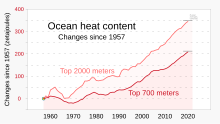
The oceans store more than 90% of the extra heat added to the climate system by Earth's energy imbalance and act as a buffer against its effects. This means that the same amount of heat that would increase the average world ocean temperature by 0.01 °C (0.018 °F) would increase atmospheric temperature by approximately 10 °C (18 °F). So a small change in the mean temperature of the ocean represents a very large change in the total heat content of the climate system. Winds and currents move heat into deeper parts of the ocean. Some of it reaches depths of more than 2,000 m (6,600 ft).
When the ocean gains heat, the water expands and sea level rises. Warmer water and water under great pressure (due to depth) expand more than cooler water and water under less pressure. Consequently, cold Arctic Ocean water will expand less than warm tropical water. Different climate models present slightly different patterns of ocean heating. So their projections do not agree fully on how much ocean heating contributes to sea level rise.
Antarctic ice loss


The large volume of ice on the Antarctic continent stores around 60% of the world's fresh water. Excluding groundwater this is 90%. Antarctica is experiencing ice loss from coastal glaciers in the West Antarctica and some glaciers of East Antarctica. However it is gaining mass from the increased snow build-up inland, particularly in the East. This leads to contradicting trends. There are different satellite methods for measuring ice mass and change. Combining them helps to reconcile the differences. However, there can still be variations between the studies. In 2018, a systematic review estimated average annual ice loss of 43 billion tons (Gt) across the entire continent between 1992 and 2002. This tripled to an annual average of 220 Gt from 2012 to 2017. However, a 2021 analysis of data from four different research satellite systems (Envisat, European Remote-Sensing Satellite, GRACE and GRACE-FO and ICESat) indicated annual mass loss of only about 12 Gt from 2012 to 2016. This was due to greater ice gain in East Antarctica than estimated earlier.
In the future, it is known that West Antarctica at least will continue to lose mass, and the likely future losses of sea ice and ice shelves, which block warmer currents from direct contact with the ice sheet, can accelerate declines even in East Antarctica. Altogether, Antarctica is the source of the largest uncertainty for future sea level projections. In 2019, the SROCC assessed several studies attempting to estimate 2300 sea level rise caused by ice loss in Antarctica alone, arriving at projected estimates of 0.07–0.37 metres (0.23–1.21 ft) for the low emission RCP2.6 scenario, and 0.60–2.89 metres (2.0–9.5 ft) in the high emission RCP8.5 scenario. However, the report notes the wide range of estimates, and gives low confidence in the projection, saying that it retains "deep uncertainty" in their ability to estimate the whole of long term damage to Antarctic ice, especially in scenarios of very high emissions.
East Antarctica
The world's largest potential source of sea level rise is the East Antarctic Ice Sheet (EAIS). It is 2.2 km thick on average and holds enough ice to raise global sea levels by 53.3 m (174 ft 10 in) Its great thickness and high elevation make it more stable than the other ice sheets. As of the early 2020s, most studies show that it is still gaining mass. Some analyses have suggested it began to lose mass in the 2000s. However they over-extrapolated some observed losses on to the poorly observed areas. A more complete observational record shows continued mass gain.

In spite of the net mass gain, some East Antarctica glaciers have lost ice in recent decades due to ocean warming and declining structural support from the local sea ice, such as Denman Glacier, and Totten Glacier. Totten Glacier is particularly important because it stabilizes the Aurora Subglacial Basin. Subglacial basins like Aurora and Wilkes Basin are major ice reservoirs together holding as much ice as all of West Antarctica. They are more vulnerable than the rest of East Antarctica. Their collective tipping point probably lies at around 3 °C (5.4 °F) of global warming. It may be as high as 6 °C (11 °F) or as low as 2 °C (3.6 °F). Once this tipping point is crossed, the collapse of these subglacial basins could take place over as little as 500 or as much as 10,000 years. The median timeline is 2000 years. Depending on how many subglacial basins are vulnerable, this causes sea level rise of between 1.4 m (4 ft 7 in) and 6.4 m (21 ft 0 in).
On the other hand, the whole EAIS would not definitely collapse until global warming reaches 7.5 °C (13.5 °F), with a range between 5 °C (9.0 °F) and 10 °C (18 °F). It would take at least 10,000 years to disappear. Some scientists have estimated that warming would have to reach at least 6 °C (11 °F) to melt two thirds of its volume.
West Antarctica
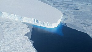
East Antarctica contains the largest potential source of sea level rise. However the West Antarctic ice sheet (WAIS) is substantially more vulnerable. Temperatures on West Antarctica have increased significantly, unlike East Antarctica and the Antarctic Peninsula. The trend is between 0.08 °C (0.14 °F) and 0.96 °C (1.73 °F) per decade between 1976 and 2012. Satellite observations recorded a substantial increase in WAIS melting from 1992 to 2017. This resulted in 7.6 ± 3.9 mm (19⁄64 ± 5⁄32 in) of Antarctica sea level rise. Outflow glaciers in the Amundsen Sea Embayment played a disproportionate role.
Scientists estimated in 2021 that the median increase in sea level rise from Antarctica by 2100 is ~11 cm (5 in). There is no difference between scenarios, because the increased warming would intensify the water cycle and increase snowfall accumulation over the EAIS at about the same rate as it would increase ice loss from WAIS. However, most of the bedrock underlying the WAIS lies well below sea level, and it has to be buttressed by the Thwaites and Pine Island glaciers. If these glaciers were to collapse, the entire ice sheet would as well. Their disappearance would take at least several centuries, but is considered almost inevitable, as their bedrock topography deepens inland and becomes more vulnerable to meltwater.
The contribution of these glaciers to global sea levels has already accelerated since the beginning of the 21st century. The Thwaites Glacier now accounts for 4% of global sea level rise. It could start to lose even more ice if the Thwaites Ice Shelf fails, potentially in mid-2020s. This is due to marine ice sheet instability hypothesis, where warm water enters between the seafloor and the base of the ice sheet once it is no longer heavy enough to displace the flow, causing accelerated melting and collapse.
Other hard-to-model processes include hydrofracturing, where meltwater collects atop the ice sheet, pools into fractures and forces them open. and changes in the ocean circulation at a smaller scale. A combination of these processes could cause the WAIS to contribute up to 41 cm (16 in) by 2100 under the low-emission scenario and up to 57 cm (22 in) under the highest-emission one.
The melting of all the ice in West Antarctica would increase the total sea level rise to 4.3 m (14 ft 1 in). However, mountain ice caps not in contact with water are less vulnerable than the majority of the ice sheet, which is located below the sea level. Its collapse would cause ~3.3 m (10 ft 10 in) of sea level rise. This collapse is now considered practically inevitable, as it appears to have already occurred during the Eemian period 125,000 years ago, when temperatures were similar to the early 21st century. This disappearance would take an estimated 2000 years. The absolute minimum for the loss of West Antarctica ice is 500 years, and the potential maximum is 13,000 years.
The only way to stop ice loss from West Antarctica once triggered is by lowering the global temperature to 1 °C (1.8 °F) below the preindustrial level. This would be 2 °C (3.6 °F) below the temperature of 2020. Other researchers suggested that a climate engineering intervention to stabilize the ice sheet's glaciers may delay its loss by centuries and give more time to adapt. However this is an uncertain proposal, and would end up as one of the most expensive projects ever attempted.
Isostatic rebound
2021 research indicates that isostatic rebound after the loss of the main portion of the West Antarctic ice sheet would ultimately add another 1.02 m (3 ft 4 in) to global sea levels. This effect would start to increase sea levels before 2100. However it would take 1000 years for it to cause 83 cm (2 ft 9 in) of sea level rise. At this point, West Antarctica itself would be 610 m (2,001 ft 4 in) higher than now. Estimates of isostatic rebound after the loss of East Antarctica's subglacial basins suggest increases of between 8 cm (3.1 in) and 57 cm (1 ft 10 in)
Greenland ice sheet loss

Most ice on Greenland is in the Greenland ice sheet which is 3 km (10,000 ft) at its thickest. The rest of Greenland ice forms isolated glaciers and ice caps. The average annual ice loss in Greenland more than doubled in the early 21st century compared to the 20th century. Its contribution to sea level rise correspondingly increased from 0.07 mm per year between 1992 and 1997 to 0.68 mm per year between 2012 and 2017. Total ice loss from the Greenland ice sheet between 1992 and 2018 amounted to 3,902 gigatons (Gt) of ice. This is equivalent to a SLR contribution of 10.8 mm. The contribution for the 2012–2016 period was equivalent to 37% of sea level rise from land ice sources (excluding thermal expansion). This observed rate of ice sheet melting is at the higher end of predictions from past IPCC assessment reports.
In 2021, AR6 estimated that by 2100, the melting of Greenland ice sheet would most likely add around 6 cm (2+1⁄2 in) to sea levels under the low-emission scenario, and 13 cm (5 in) under the high-emission scenario. The first scenario, SSP1-2.6, largely fulfils the Paris Agreement goals, while the other, SSP5-8.5, has the emissions accelerate throughout the century. The uncertainty about ice sheet dynamics can affect both pathways. In the best-case scenario, ice sheet under SSP1-2.6 gains enough mass by 2100 through surface mass balance feedbacks to reduce the sea levels by 2 cm (1 in). In the worst case, it adds 15 cm (6 in). For SSP5-8.5, the best-case scenario is adding 5 cm (2 in) to sea levels, and the worst-case is adding 23 cm (9 in)
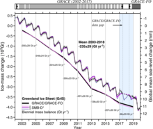
Greenland's peripheral glaciers and ice caps crossed an irreversible tipping point around 1997. Sea level rise from their loss is now unstoppable. However the temperature changes in future, the warming of 2000–2019 had already damaged the ice sheet enough for it to eventually lose ~3.3% of its volume. This is leading to 27 cm (10+1⁄2 in) of future sea level rise. At a certain level of global warming, the Greenland ice sheet will almost completely melt. Ice cores show this happened at least once during the last million years, when the temperatures have at most been 2.5 °C (4.5 °F) warmer than the preindustrial.
2012 research suggested that the tipping point of the ice sheet was between 0.8 °C (1.4 °F) and 3.2 °C (5.8 °F). 2023 modelling has narrowed the tipping threshold to a 1.7 °C (3.1 °F)-2.3 °C (4.1 °F) range. If temperatures reach or exceed that level, reducing the global temperature to 1.5 °C (2.7 °F) above pre-industrial levels or lower would prevent the loss of the entire ice sheet. One way to do this in theory would be large-scale carbon dioxide removal. But it would also cause greater losses and sea level rise from Greenland than if the threshold was not breached in the first place. Otherwise, the ice sheet would take between 10,000 and 15,000 years to disintegrate entirely once the tipping point had been crossed. The most likely estimate is 10,000 years. If climate change continues along its worst trajectory and temperatures continue to rise quickly over multiple centuries, it would only take 1,000 years.
Mountain glacier loss

There are roughly 200,000 glaciers on Earth, which are spread out across all continents. Less than 1% of glacier ice is in mountain glaciers, compared to 99% in Greenland and Antarctica. However, this small size also makes mountain glaciers more vulnerable to melting than the larger ice sheets. This means they have had a disproportionate contribution to historical sea level rise and are set to contribute a smaller, but still significant fraction of sea level rise in the 21st century. Observational and modelling studies of mass loss from glaciers and ice caps show they contribute 0.2-0.4 mm per year to sea level rise, averaged over the 20th century. The contribution for the 2012–2016 period was nearly as large as that of Greenland. It was 0.63 mm of sea level rise per year, equivalent to 34% of sea level rise from land ice sources. Glaciers contributed around 40% to sea level rise during the 20th century, with estimates for the 21st century of around 30%.
In 2023, a Science paper estimated that at 1.5 °C (2.7 °F), one quarter of mountain glacier mass would be lost by 2100 and nearly half would be lost at 4 °C (7.2 °F), contributing ~9 cm (3+1⁄2 in) and ~15 cm (6 in) to sea level rise, respectively. Glacier mass is disproportionately concentrated in the most resilient glaciers. So in practice this would remove 49-83% of glacier formations. It further estimated that the current likely trajectory of 2.7 °C (4.9 °F) would result in the SLR contribution of ~11 cm (4+1⁄2 in) by 2100. Mountain glaciers are even more vulnerable over the longer term. In 2022, another Science paper estimated that almost no mountain glaciers could survive once warming crosses 2 °C (3.6 °F). Their complete loss is largely inevitable around 3 °C (5.4 °F). There is even a possibility of complete loss after 2100 at just 1.5 °C (2.7 °F). This could happen as early as 50 years after the tipping point is crossed, although 200 years is the most likely value, and the maximum is around 1000 years.
Sea ice loss
Sea ice loss contributes very slightly to global sea level rise. If the melt water from ice floating in the sea was exactly the same as sea water then, according to Archimedes' principle, no rise would occur. However melted sea ice contains less dissolved salt than sea water and is therefore less dense, with a slightly greater volume per unit of mass. If all floating ice shelves and icebergs were to melt sea level would only rise by about 4 cm (1+1⁄2 in).

Changes to land water storage
Human activity impacts how much water is stored on land. Dams retain large quantities of water, which is stored on land rather than flowing into the sea, though the total quantity stored will vary from time to time. On the other hand, humans extract water from lakes, wetlands and underground reservoirs for food production. This often causes subsidence. Furthermore, the hydrological cycle is influenced by climate change and deforestation. This can increase or reduce contributions to sea level rise. In the 20th century, these processes roughly balanced, but dam building has slowed down and is expected to stay low for the 21st century.
Water redistribution caused by irrigation from 1993 to 2010 caused a drift of Earth's rotational pole by 78.48 centimetres (30.90 in). This caused groundwater depletion equivalent to a global sea level rise of 6.24 millimetres (0.246 in).
Impacts
On people and societies

Sea-level rise has many impacts. They include higher and more frequent high-tide and storm-surge flooding and increased coastal erosion. Other impacts are inhibition of primary production processes, more extensive coastal inundation, and changes in surface water quality and groundwater. These can lead to a greater loss of property and coastal habitats, loss of life during floods and loss of cultural resources. There are also impacts on agriculture and aquaculture. There can also be loss of tourism, recreation, and transport-related functions. Land use changes such as urbanisation or deforestation of low-lying coastal zones exacerbate coastal flooding impacts. Regions already vulnerable to rising sea level also struggle with coastal flooding. This washes away land and alters the landscape.
Changes in emissions are likely to have only a small effect on the extent of sea level rise by 2050. So projected sea level rise could put tens of millions of people at risk by then. Scientists estimate that 2050 levels of sea level rise would result in about 150 million people under the water line during high tide. About 300 million would be in places flooded every year. This projection is based on the distribution of population in 2010. It does not take into account the effects of population growth and human migration. These figures are 40 million and 50 million more respectively than the numbers at risk in 2010. By 2100, there would be another 40 million people under the water line during high tide if sea level rise remains low. This figure would be 80 million for a high estimate of median sea level rise. Ice sheet processes under the highest emission scenario would result in sea level rise of well over one metre (3+1⁄4 ft) by 2100. This could be as much as over two metres (6+1⁄2 ft), This could result in as many as 520 million additional people ending up under the water line during high tide and 640 million in places flooded every year, compared to the 2010 population distribution.

Over the longer term, coastal areas are particularly vulnerable to rising sea levels. They are also vulnerable to changes in the frequency and intensity of storms, increased precipitation, and rising ocean temperatures. Ten percent of the world's population live in coastal areas that are less than 10 metres (33 ft) above sea level. Two thirds of the world's cities with over five million people are located in these low-lying coastal areas. About 600 million people live directly on the coast around the world. Cities such as Miami, Rio de Janeiro, Osaka and Shanghai will be especially vulnerable later in the century under warming of 3 °C (5.4 °F). This is close to the current trajectory. LiDAR-based research had established in 2021 that 267 million people worldwide lived on land less than 2 m (6+1⁄2 ft) above sea level. With a 1 m (3+1⁄2 ft) sea level rise and zero population growth, that could increase to 410 million people.
Potential disruption of sea trade and migrations could impact people living further inland. United Nations Secretary-General António Guterres warned in 2023 that sea level rise risks causing human migrations on a "biblical scale". Sea level rise will inevitably affect ports, but there is limited research on this. There is insufficient knowledge about the investments necessary to protect ports currently in use. This includes protecting current facilities before it becomes more reasonable to build new ports elsewhere. Some coastal regions are rich agricultural lands. Their loss to the sea could cause food shortages. This is a particularly acute issue for river deltas such as Nile Delta in Egypt and Red River and Mekong Deltas in Vietnam. Saltwater intrusion into the soil and irrigation water has a disproportionate effect on them.
On ecosystems

Flooding and soil/water salinization threaten the habitats of coastal plants, birds, and freshwater/estuarine fish when seawater reaches inland. When coastal forest areas become inundated with saltwater to the point no trees can survive the resulting habitats are called ghost forests. Starting around 2050, some nesting sites in Florida, Cuba, Ecuador and the island of Sint Eustatius for leatherback, loggerhead, hawksbill, green and olive ridley turtles are expected to be flooded. The proportion will increase over time. In 2016, Bramble Cay islet in the Great Barrier Reef was inundated. This flooded the habitat of a rodent named Bramble Cay melomys. It was officially declared extinct in 2019.
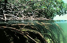
Some ecosystems can move inland with the high-water mark. But natural or artificial barriers prevent many from migrating. This coastal narrowing is sometimes called 'coastal squeeze' when it involves human-made barriers. It could result in the loss of habitats such as mudflats and tidal marshes. Mangrove ecosystems on the mudflats of tropical coasts nurture high biodiversity. They are particularly vulnerable due to mangrove plants' reliance on breathing roots or pneumatophores. These will be submerged if the rate is too rapid for them to migrate upward. This would result in the loss of an ecosystem. Both mangroves and tidal marshes protect against storm surges, waves and tsunamis, so their loss makes the effects of sea level rise worse. Human activities such as dam building may restrict sediment supplies to wetlands. This would prevent natural adaptation processes. The loss of some tidal marshes is unavoidable as a consequence.
Corals are important for bird and fish life. They need to grow vertically to remain close to the sea surface in order to get enough energy from sunlight. The corals have so far been able to keep up the vertical growth with the rising seas, but might not be able to do so in the future.
Adaptation

Cutting greenhouse gas emissions can slow and stabilize the rate of sea level rise after 2050. This would greatly reduce its costs and damages, but cannot stop it outright. So climate change adaptation to sea level rise is inevitable. The simplest approach is to stop development in vulnerable areas and ultimately move people and infrastructure away from them. Such retreat from sea level rise often results in the loss of livelihoods. The displacement of newly impoverished people could burden their new homes and accelerate social tensions.
It is possible to avoid or at least delay the retreat from sea level rise with enhanced protections. These include dams, levees or improved natural defenses. Other options include updating building standards to reduce damage from floods, addition of storm water valves to address more frequent and severe flooding at high tide, or cultivating crops more tolerant of saltwater in the soil, even at an increased cost. These options divide into hard and soft adaptation. Hard adaptation generally involves large-scale changes to human societies and ecological systems. It often includes the construction of capital-intensive infrastructure. Soft adaptation involves strengthening natural defenses and local community adaptation. This usually involves simple, modular and locally owned technology. The two types of adaptation may be complementary or mutually exclusive. Adaptation options often require significant investment. But the costs of doing nothing are far greater. One example would involve adaptation against flooding. Effective adaptation measures could reduce future annual costs of flooding in 136 of the world's largest coastal cities from $1 trillion by 2050 without adaptation to a little over $60 billion annually. The cost would be $50 billion per year. Some experts argue that retreat from the coast would have a lower impact on the GDP of India and Southeast Asia then attempting to protect every coastline, in the case of very high sea level rise.

To be successful, adaptation must anticipate sea level rise well ahead of time. As of 2023, the global state of adaptation planning is mixed. A survey of 253 planners from 49 countries found that 98% are aware of sea level rise projections, but 26% have not yet formally integrated them into their policy documents. Only around a third of respondents from Asian and South American countries have done so. This compares with 50% in Africa, and over 75% in Europe, Australasia and North America. Some 56% of all surveyed planners have plans which account for 2050 and 2100 sea level rise. But 53% use only a single projection rather than a range of two or three projections. Just 14% use four projections, including the one for "extreme" or "high-end" sea level rise. Another study found that over 75% of regional sea level rise assessments from the West and Northeastern United States included at least three estimates. These are usually RCP2.6, RCP4.5 and RCP8.5, and sometimes include extreme scenarios. But 88% of projections from the American South had only a single estimate. Similarly, no assessment from the South went beyond 2100. By contrast 14 assessments from the West went up to 2150, and three from the Northeast went to 2200. 56% of all localities were also found to underestimate the upper end of sea level rise relative to IPCC Sixth Assessment Report.
By region
Africa

In Africa, future population growth amplifies risks from sea level rise. Some 54.2 million people lived in the highly exposed low elevation coastal zones (LECZ) around 2000. This number will effectively double to around 110 million people by 2030, and then reach 185 to 230 million people by 2060. By then, the average regional sea level rise will be around 21 cm, with little difference from climate change scenarios. By 2100, Egypt, Mozambique and Tanzania are likely to have the largest number of people affected by annual flooding amongst all African countries. And under RCP8.5, 10 important cultural sites would be at risk of flooding and erosion by the end of the century.
In the near term, some of the largest displacement is projected to occur in the East Africa region. At least 750,000 people there are likely to be displaced from the coasts between 2020 and 2050. By 2050, 12 major African cities would collectively sustain cumulative damages of US$65 billion for the "moderate" climate change scenario RCP4.5 and between US$86.5 billion to US$137.5 billion on average: in the worst case, these damages could effectively triple. In all of these estimates, around half of the damages would occur in the Egyptian city of Alexandria. Hundreds of thousands of people in its low-lying areas may already need relocation in the coming decade. Across sub-Saharan Africa as a whole, damage from sea level rise could reach 2–4% of GDP by 2050, although this depends on the extent of future economic growth and climate change adaptation.
Asia


Asia has the largest population at risk from sea level due to its dense coastal populations. As of 2022, some 63 million people in East and South Asia were already at risk from a 100-year flood. This is largely due to inadequate coastal protection in many countries. Bangladesh, China, India, Indonesia, Japan, Pakistan, the Philippines, Thailand and Vietnam alone account for 70% of people exposed to sea level rise during the 21st century. Sea level rise in Bangladesh is likely to displace 0.9-2.1 million people by 2050. It may also force the relocation of up to one third of power plants as early as 2030, and many of the remaining plants would have to deal with the increased salinity of their cooling water. Nations like Bangladesh, Vietnam and China with extensive rice production on the coast are already seeing adverse impacts from saltwater intrusion.
Modelling results predict that Asia will suffer direct economic damages of US$167.6 billion at 0.47 meters of sea level rise. This rises to US$272.3 billion at 1.12 meters and US$338.1 billion at 1.75 meters. There is an additional indirect impact of US$8.5, 24 or 15 billion from population displacement at those levels. China, India, the Republic of Korea, Japan, Indonesia and Russia experience the largest economic losses. Out of the 20 coastal cities expected to see the highest flood losses by 2050, 13 are in Asia. Nine of these are the so-called sinking cities, where subsidence (typically caused by unsustainable groundwater extraction in the past) would compound sea level rise. These are Bangkok, Guangzhou, Ho Chi Minh City, Jakarta, Kolkata, Nagoya, Tianjin, Xiamen and Zhanjiang.
By 2050, Guangzhou would see 0.2 meters of sea level rise and estimated annual economic losses of US$254 million – the highest in the world. In Shanghai, coastal inundation amounts to about 0.03% of local GDP, yet would increase to 0.8% by 2100 even under the "moderate" RCP4.5 scenario in the absence of adaptation. The city of Jakarta is sinking so much (up to 28 cm (11 in) per year between 1982 and 2010 in some areas) that in 2019, the government had committed to relocate the capital of Indonesia to another city.
Australasia

In Australia, erosion and flooding of Queensland's Sunshine Coast beaches is likely to intensify by 60% by 2030. Without adaptation there would be a big impact on tourism. Adaptation costs for sea level rise would be three times higher under the high-emission RCP8.5 scenario than in the low-emission RCP2.6 scenario. Sea level rise of 0.2-0.3 meters is likely by 2050. In these conditions what is currently a 100-year flood would occur every year in the New Zealand cities of Wellington and Christchurch. With 0.5 m sea level rise, a current 100-year flood in Australia would occur several times a year. In New Zealand this would expose buildings with a collective worth of NZ$12.75 billion to new 100-year floods. A meter or so of sea level rise would threaten assets in New Zealand with a worth of NZD$25.5 billion. There would be a disproportionate impact on Maori-owned holdings and cultural heritage objects. Australian assets worth AUS$164–226 billion including many unsealed roads and railway lines would also be at risk. This amounts to a 111% rise in Australia's inundation costs between 2020 and 2100.
Central and South America
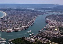
By 2100, coastal flooding and erosion will affect at least 3-4 million people in South America. Many people live in low-lying areas exposed to sea level rise. This includes 6% of the population of Venezuela, 56% of the population of Guyana and 68% of the population of Suriname. In Guyana much of the capital Georgetown is already below sea level. In Brazil, the coastal ecoregion of Caatinga is responsible for 99% of its shrimp production. A combination of sea level rise, ocean warming and ocean acidification threaten its unique. Extreme wave or wind behavior disrupted the port complex of Santa Catarina 76 times in one 6-year period in the 2010s. There was a US$25,000-50,000 loss for each idle day. In Port of Santos, storm surges were three times more frequent between 2000 and 2016 than between 1928 and 1999.
Europe

Many sandy coastlines in Europe are vulnerable to erosion due to sea level rise. In Spain, Costa del Maresme is likely to retreat by 16 meters by 2050 relative to 2010. This could amount to 52 meters by 2100 under RCP8.5 Other vulnerable coastlines include the Tyrrhenian Sea coast of Italy's Calabria region, the Barra-Vagueira coast in Portugal and Nørlev Strand in Denmark.
In France, it was estimated that 8,000-10,000 people would be forced to migrate away from the coasts by 2080. The Italian city of Venice is located on islands. It is highly vulnerable to flooding and has already spent $6 billion on a barrier system. A quarter of the German state of Schleswig-Holstein, inhabited by over 350,000 people, is at low elevation and has been vulnerable to flooding since preindustrial times. Many levees already exist. Because of its complex geography, the authorities chose a flexible mix of hard and soft measures to cope with sea level rise of over 1 meter per century. In the United Kingdom, sea level at the end of the century would increase by 53 to 115 centimeters at the mouth of the River Thames and 30 to 90 centimeters at Edinburgh. The UK has divided its coast into 22 areas, each covered by a Shoreline Management Plan. Those are sub-divided into 2000 management units, working across three periods of 0–20, 20-50 and 50–100 years.
The Netherlands is a country that sits partially below sea level and is subsiding. It has responded by extending its Delta Works program. Drafted in 2008, the Delta Commission report said that the country must plan for a rise in the North Sea up to 1.3 m (4 ft 3 in) by 2100 and plan for a 2–4 m (7–13 ft) rise by 2200. It advised annual spending between €1.0 and €1.5 billion. This would support measures such as broadening coastal dunes and strengthening sea and river dikes. Worst-case evacuation plans were also drawn up.
North America

As of 2017, around 95 million Americans lived on the coast. The figures for Canada and Mexico were 6.5 million and 19 million. Increased chronic nuisance flooding and king tide flooding is already a problem in the highly vulnerable state of Florida. The US East Coast is also vulnerable. On average, the number of days with tidal flooding in the US increased 2 times in the years 2000–2020, reaching 3–7 days per year. In some areas the increase was much stronger: 4 times in the Southeast Atlantic and 11 times in the Western Gulf. By the year 2030 the average number is expected to be 7–15 days, reaching 25–75 days by 2050. U.S. coastal cities have responded with beach nourishment or beach replenishment. This trucks in mined sand in addition to other adaptation measures such as zoning, restrictions on state funding, and building code standards. Along an estimated some 15% of the US coastline, the majority of local groundwater levels are already below sea level. This places those groundwater reservoirs at risk of sea water intrusion. That would render fresh water unusable once its concentration exceeds 2-3%. Damage is also widespread in Canada. It will affect major cities like Halifax and more remote locations like Lennox Island. The Mi'kmaq community there is already considering relocation due to widespread coastal erosion. In Mexico, damage from SLR to tourism hotspots like Cancun, Isla Mujeres, Playa del Carmen, Puerto Morelos and Cozumel could amount to US$1.4–2.3 billion. The increase in storm surge due to sea level rise is also a problem. Due to this effect Hurricane Sandy caused an additional US$8 billion in damage, impacted 36,000 more houses and 71,000 more people.
In future, the northern Gulf of Mexico, Atlantic Canada and the Pacific coast of Mexico would experience the greatest sea level rise. By 2030, flooding along the US Gulf Coast could cause economic losses of up to US$176 billion. Using nature-based solutions like wetland restoration and oyster reef restoration could avoid around US$50 billion of this. By 2050, coastal flooding in the US is likely to rise tenfold to four "moderate" flooding events per year. That forecast is even without storms or heavy rainfall. In New York City, current 100-year flood would occur once in 19–68 years by 2050 and 4–60 years by 2080. By 2050, 20 million people in the greater New York City area would be at risk. This is because 40% of existing water treatment facilities would be compromised and 60% of power plants will need relocation. By 2100, sea level rise of 0.9 m (3 ft) and 1.8 m (6 ft) would threaten 4.2 and 13.1 million people in the US, respectively. In California alone, 2 m (6+1⁄2 ft) of SLR could affect 600,000 people and threaten over US$150 billion in property with inundation. This potentially represents over 6% of the state's GDP. In North Carolina, a meter of SLR inundates 42% of the Albemarle-Pamlico Peninsula, costing up to US$14 billion. In nine southeast US states, the same level of sea level rise would claim up to 13,000 historical and archaeological sites, including over 1000 sites eligible for inclusion in the National Register for Historic Places.
Island nations

Small island states are nations with populations on atolls and other low islands. Atolls on average reach 0.9–1.8 m (3–6 ft) above sea level. These are the most vulnerable places to coastal erosion, flooding and salt intrusion into soils and freshwater caused by sea level rise. Sea level rise may make an island uninhabitable before it is completely flooded. Already, children in small island states encounter hampered access to food and water. They suffer an increased rate of mental and social disorders due to these stresses. At current rates, sea level rise would be high enough to make the Maldives uninhabitable by 2100. Five of the Solomon Islands have already disappeared due to the effects of sea level rise and stronger trade winds pushing water into the Western Pacific.
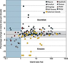
Adaptation to sea level rise is costly for small island nations as a large portion of their population lives in areas that are at risk. Nations like Maldives, Kiribati and Tuvalu already have to consider controlled international migration of their population in response to rising seas. The alternative of uncontrolled migration threatens to worsen the humanitarian crisis of climate refugees. In 2014, Kiribati purchased 20 square kilometers of land (about 2.5% of Kiribati's current area) on the Fijian island of Vanua Levu to relocate its population once their own islands are lost to the sea.
Fiji also suffers from sea level rise. It is in a comparatively safer position. Its residents continue to rely on local adaptation like moving further inland and increasing sediment supply to combat erosion instead of relocating entirely. Fiji has also issued a green bond of $50 million to invest in green initiatives and fund adaptation efforts. It is restoring coral reefs and mangroves to protect against flooding and erosion. It sees this as a more cost-efficient alternative to building sea walls. The nations of Palau and Tonga are taking similar steps. Even when an island is not threatened with complete disappearance from flooding, tourism and local economies may end up devastated. For instance, sea level rise of 1.0 m (3 ft 3 in) would cause partial or complete inundation of 29% of coastal resorts in the Caribbean. A further 49–60% of coastal resorts would be at risk from resulting coastal erosion.
