If you are reading this, you probably had a linear algebra class and remember your professor mentioning two strange words: Eigenvector and Eigenvalue. Maybe you remember the equation. However, WHAT ARE THEY?
The best short definition that I can give is:
“Eigenvectors are the vectors that stay parallel after a matrix transformation”
Still confused? I am sure you’ll understand by the end of this article.

In words, we want to find the scalar lambda “λ” and the nonzero vector “v” such that the equation holds.
Let’s do some algebraic magic to find a solution. In order to solve the equation as a matrix subtraction, we want to use the IDENTITY matrix as follows:
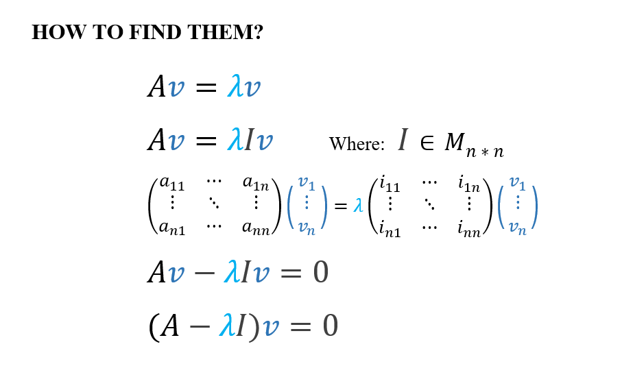
Since we established the vector “v” is not the trivial solution (zero vector), we will use the DETERMINANT as a tool.

In other words, we know that if a square matrix has a zero determinant, it has an infinite number of solutions. Thus, the eigenvalues are the lambda “λ” scalars for which the matrix below has a zero determinant:

Once we calculate these special values (eigenvalues), we can find the associated eigenvectors to each eigenvalue.
Let’s work on an example to see what this is all about!

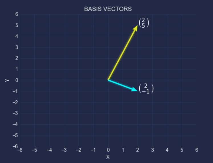
- This, is a graphical representation of matrix “A” by its decomposition into two different vectors (basis vectors):
- We use the identity matrix to solve for the eigenvalues:
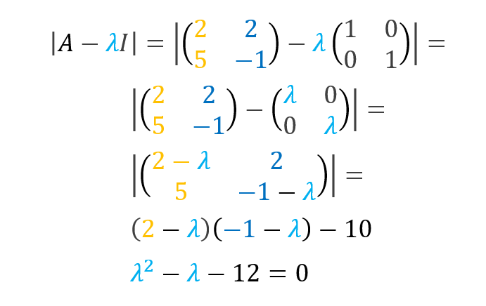
At this point, we have to use the quadratic equation to get the values for lambda “λ”:

If you don’t remember how to calculate the determinant of a matrix, you can check this post: “Determinant of a matrix”
Before calculating the eigenvalues, we need to grasp the concept of matrices as a transformation of vectors and the Cartesian Plane (This VIDEO explains well the graphical meaning of matrices as linear transformations and how seeing them in action helps to understand linear algebra better).

……………………………
“Unfortunately, no one can be told what the Matrix is. You have to see it for yourself”
- Morpheus
…………………………………..
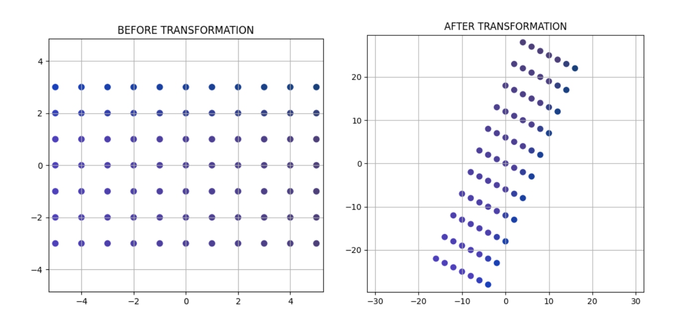
Thus, let me show you a matrix:
As you can see in the picture below, a matrix transforms all the points in the plane (represented as vectors with coordinates in the X and Y axis for the 2D case).
Continuing with the example…
Now, we can find the eigenvectors using the initial equation:
- For lambda(1) “λ(1)” = -3

In fact, the eigenvector associated with -3 is any non-zero multiple of the “e(1)”. Thus, “e(1)” spans the set of eigenvectors associated with the eigenvalue “λ(1)” -3.


- For lambda(2) “λ(2)” = 4
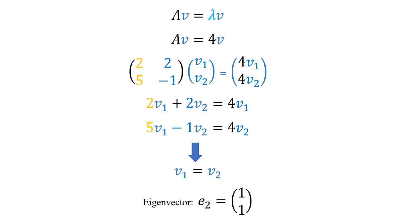
In the same manner, the eigenvector associated with 4 is any non-zero multiple of “e(2)”. Thus, “e(2)” spans the set of eigenvectors associated with the eigenvalue “λ(2)” 4.


- Finally, let’s see what happens when we transform any vector other than vectors from the span of “e(1)” and “e(2)”:


As you can see: The vector didn’t stay parallel after the transformation and that’s why it’s not an eigenvector!
