From Wikipedia, the free encyclopedia
The Clausius–Clapeyron relation, named after Rudolf Clausius[1] and Benoît Paul Émile Clapeyron,[2] is a way of characterizing a discontinuous phase transition between two phases of matter of a single constituent. On a pressure–temperature (P–T) diagram, the line separating the two phases is known as the coexistence curve. The Clausius–Clapeyron relation gives the slope of the tangents to this curve. Mathematically,
 is the slope of the tangent to the coexistence curve at any point,
  is the specific latent heat,
  is the temperature,
  is the specific volume change of the phase transition and
  is the entropy change of the phase transition.
 for a homogeneous substance to be a function of specific volume
  and temperature .[3]:508
 is the pressure. Since pressure and temperature are constant, by definition the derivative of pressure with respect to temperature does not change.[4][5]:57, 62 & 671 Therefore the partial derivative of specific entropy may be changed into a total derivative
 to a final phase
  ,[3]:508 to obtain
 and
and  are respectively the change in specific entropy and specific volume. Given that a phase change is an internally reversible process, and that our system is closed, the first law of thermodynamics holds
 is the internal energy of the system. Given constant pressure and temperature (during a phase change) and the definition of specific enthalpy
  , we obtain
 gives
gives
 ), we obtain[3]:508[6]
, at any given point on the curve, to the function  of the specific latent heat , the temperature , and the change in specific volume .
and , are in contact and at equilibrium with each other. Their chemical potentials are related by
is the specific entropy, is the specific volume, and  is the molar mass) to obtain
 greatly exceeds that of the condensed phase
  . Therefore one may approximate
is the pressure,  is the specific gas constant, and is the temperature. Substituting into the Clapeyron equation
is the specific latent heat of the substance.
Let and
and  be any two points along the coexistence curve between two phases and . In general, varies between any two such points, as a function of temperature. But if is constant,
 is a constant. For a liquid-gas transition, is the specific latent heat (or specific enthalpy) of vaporization; for a solid-gas transition, is the specific latent heat of sublimation. If the latent heat is known, then knowledge of one point on the coexistence curve determines the rest of the curve. Conversely, the relationship between
  and
and  is linear, and so linear regression is used to estimate the latent heat.
 , and therefore of the saturation vapor pressure
  , cannot be neglected in this application. Fortunately, the August-Roche-Magnus formula provides a very good approximation, using pressure in hPa and temperature in Celsius:
(This is also sometimes called the Magnus or Magnus-Tetens approximation, though this attribution is historically inaccurate.[9])
Under typical atmospheric conditions, the denominator of the exponent depends weakly on (for which the unit is Celsius). Therefore, the August-Roche-Magnus equation implies that saturation water vapor pressure changes approximately exponentially with temperature under typical atmospheric conditions, and hence the water-holding capacity of the atmosphere increases by about 7% for every 1 °C rise in temperature.[10]
 below 0 °C. Note that water is unusual in that its change in volume upon melting is negative. We can assume
 is the specific heat capacity at constant pressure,
  is the thermal expansion coefficient, and
  is the isothermal compressibility.

 is the slope of the tangent to the coexistence curve at any point,
  is the specific latent heat,
  is the temperature,
  is the specific volume change of the phase transition and
  is the entropy change of the phase transition.
Derivations

Derivation from state postulate
Using the state postulate, take the specific entropy for a homogeneous substance to be a function of specific volume
  and temperature .[3]:508
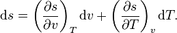


 is the pressure. Since pressure and temperature are constant, by definition the derivative of pressure with respect to temperature does not change.[4][5]:57, 62 & 671 Therefore the partial derivative of specific entropy may be changed into a total derivative
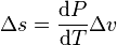
 to a final phase
  ,[3]:508 to obtain
 and
and  are respectively the change in specific entropy and specific volume. Given that a phase change is an internally reversible process, and that our system is closed, the first law of thermodynamics holds
 is the internal energy of the system. Given constant pressure and temperature (during a phase change) and the definition of specific enthalpy
  , we obtain
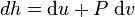


 gives
gives
 ), we obtain[3]:508[6]
 , at any given point on the curve, to the function
  of the specific latent heat , the temperature , and the change in specific volume .
Derivation from Gibbs–Duhem relation
Suppose two phases, and , are in contact and at equilibrium with each other. Their chemical potentials are related by

 is the specific entropy, is the specific volume, and
  is the molar mass) to obtain

Ideal gas approximation at low temperatures
When the phase transition of a substance is between a gas phase and a condensed phase (liquid or solid), and occurs at temperatures much lower than the critical temperature of that substance, the specific volume of the gas phase greatly exceeds that of the condensed phase
  . Therefore one may approximate
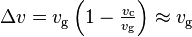
 is the pressure,
  is the specific gas constant, and is the temperature. Substituting into the Clapeyron equation
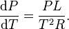 is the specific latent heat of the substance.
Let
 and
and  be any two points along the coexistence curve between two phases and . In general, varies between any two such points, as a function of temperature. But if is constant,


Applications
Chemistry and chemical engineering
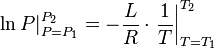
For transitions between a gas and a condensed phase with the approximations described above, the expression may be rewritten as
 is a constant. For a liquid-gas transition, is the specific latent heat (or specific enthalpy) of vaporization; for a solid-gas transition, is the specific latent heat of sublimation. If the latent heat is known, then knowledge of one point on the coexistence curve determines the rest of the curve. Conversely, the relationship between
  and
and  is linear, and so linear regression is used to estimate the latent heat.
Meteorology and climatology
Atmospheric water vapor drives many important meteorologic phenomena (notably precipitation), motivating interest in its dynamics. The Clausius–Clapeyron equation for water vapor under typical atmospheric conditions (near standard temperature and pressure) is
 is saturation vapor pressure
- is temperature
 is the specific latent heat of evaporation of water
 is the gas constant of water vapor
 is
is  is the
  is the
  , and therefore of the saturation vapor pressure
  , cannot be neglected in this application. Fortunately, the August-Roche-Magnus formula provides a very good approximation, using pressure in hPa and temperature in Celsius:
(This is also sometimes called the Magnus or Magnus-Tetens approximation, though this attribution is historically inaccurate.[9])
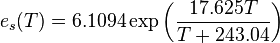
Under typical atmospheric conditions, the denominator of the exponent depends weakly on
(for which the unit is Celsius). Therefore, the August-Roche-Magnus equation implies that saturation water vapor pressure changes approximately exponentially with temperature under typical atmospheric conditions, and hence the water-holding capacity of the atmosphere increases by about 7% for every 1 °C rise in temperature.[10]Example
One of the uses of this equation is to determine if a phase transition will occur in a given situation. Consider the question of how much pressure is needed to melt ice at a temperature below 0 °C. Note that water is unusual in that its change in volume upon melting is negative. We can assume
- = 3.34×10⁵ J/kg (latent heat of fusion for water),
- = 273 K (absolute temperature), and
- = −9.05×10⁻⁵ m³/kg (change in specific volume from solid to liquid),
 = −13.5 MPa/K.
 = −13.5 MPa/K.
Second derivative
While the Clausius–Clapeyron relation gives the slope of the coexistence curve, it does not provide any information about its curvature or second derivative. The second derivative of the coexistence curve of phases 1 and 2 is given by [12]![\frac{\mathrm{d}^2 P}{\mathrm{d} T^2} = \frac{1}{v_2 - v_1}
\left[\frac{c_{p2} - c_{p1}}{T} - 2(v_2\alpha_2 - v_1\alpha_1) \frac{\mathrm{d}P}{\mathrm{d}T} + (v_2\kappa_{T2} - v_1\kappa_{T1})\left(\frac{\mathrm{d}P}{\mathrm{d}T}\right)^2\right],](http://upload.wikimedia.org/math/d/3/7/d3753e19c46436f63d271ea0b81516c4.png)
 is the specific heat capacity at constant pressure,
  is the thermal expansion coefficient, and
  is the isothermal compressibility.

