F-test

From Wikipedia, the free encyclopedia
https://en.wikipedia.org/wiki/F-test

An f-test pdf with d1 and d2 = 10, at a significance level of 0.05. (Red shaded region indicates the critical region)

An F-test is a statistical test that compares variances. It's used to determine if the variances of two samples, or if the ratios of variances among multiple samples, are significantly different. The test calculates a statistic, represented by the random variable F, and checks if it follows an F-distribution. This check is valid if the null hypothesis is true and standard assumptions about the errors (ε) in the data hold.

F-tests are frequently used to compare different statistical models and find the one that best describes the population the data came from. When models are created using the least squares method, the resulting F-tests are often called "exact" F-tests. The F-statistic was developed by Ronald Fisher in the 1920s as the variance ratio and was later named in his honor by George W. Snedecor.

Common examples

Common examples of the use of F-tests include the study of the following cases

• 

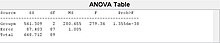
  One-way ANOVA table with 3 random groups that each has 30 observations. F value is being calculated in the second to last column

  The hypothesis that the means of a given set of normally distributed populations, all having the same standard deviation, are equal. This is perhaps the best-known F-test, and plays an important role in the analysis of variance (ANOVA).
  • F test of analysis of variance (ANOVA) follows three assumptions
    1. Normality (statistics)
    2. Homogeneity of variance
    3. Independence of errors and random sampling

• The hypothesis that a proposed regression model fits the data well. See Lack-of-fit sum of squares.
• The hypothesis that a data set in a regression analysis follows the simpler of two proposed linear models that are nested within each other.
• Multiple-comparison testing is conducted using needed data in already completed F-test, if F-test leads to rejection of null hypothesis and the factor under study has an impact on the dependent variable.
  • "a priori comparisons"/ "planned comparisons"- a particular set of comparisons
  • "pairwise comparisons"-all possible comparisons
    • i.e. Fisher's least significant difference (LSD) test, Tukey's honestly significant difference (HSD) test, Newman Keuls test, Ducan's test
  • "a posteriori comparisons"/ "post hoc comparisons"/ "exploratory comparisons"- choose comparisons after examining the data
    • i.e. Scheffé's method

F-test of the equality of two variances

Main article: F-test of equality of variances

The F-test is sensitive to non-normality. In the analysis of variance (ANOVA), alternative tests include Levene's test, Bartlett's test, and the Brown–Forsythe test. However, when any of these tests are conducted to test the underlying assumption of homoscedasticity (i.e. homogeneity of variance), as a preliminary step to testing for mean effects, there is an increase in the experiment-wise Type I error rate.

Formula and calculation

Most F-tests arise by considering a decomposition of the variability in a collection of data in terms of sums of squares. The test statistic in an F-test is the ratio of two scaled sums of squares reflecting different sources of variability. These sums of squares are constructed so that the statistic tends to be greater when the null hypothesis is not true. In order for the statistic to follow the F-distribution under the null hypothesis, the sums of squares should be statistically independent, and each should follow a scaled χ²-distribution. The latter condition is guaranteed if the data values are independent and normally distributed with a common variance.

One-way analysis of variance

The formula for the one-way ANOVA F-test statistic is

${\displaystyle F=\frac{\text{explained variance}}{\text{unexplained variance}},}$

or

${\displaystyle F=\frac{\text{between-group variability}}{\text{within-group variability}}.}$

The "explained variance", or "between-group variability" is

${\displaystyle \sum _{i=1}^K{n}_i({\overline{Y}}_{i\cdot }-\overline{Y}{)}^2/(K-1)}$

where ${\displaystyle {\overline{Y}}_{i\cdot }}$ denotes the sample mean in the i-th group, ${\displaystyle n_i}$ is the number of observations in the i-th group, ${\displaystyle \overline{Y}}$ denotes the overall mean of the data, and ${\displaystyle K}$ denotes the number of groups.

The "unexplained variance", or "within-group variability" is

${\displaystyle \sum _{i=1}^K\sum _{j=1}^{n_i}{\left(Y_{ij}-{\overline{Y}}_{i\cdot }\right)}^2/(N-K),}$

where ${\displaystyle Y_{ij}}$ is the j^th observation in the i^th out of ${\displaystyle K}$ groups and ${\displaystyle N}$ is the overall sample size. This F-statistic follows the F-distribution with degrees of freedom ${\displaystyle d_1=K-1}$ and ${\displaystyle d_2=N-K}$ under the null hypothesis. The statistic will be large if the between-group variability is large relative to the within-group variability, which is unlikely to happen if the population means of the groups all have the same value.

F Table: Level 5% Critical values, containing degrees of freedoms for both denominator and numerator ranging from 1-20

The result of the F test can be determined by comparing calculated F value and critical F value with specific significance level (e.g. 5%). The F table serves as a reference guide containing critical F values for the distribution of the F-statistic under the assumption of a true null hypothesis. It is designed to help determine the threshold beyond which the F statistic is expected to exceed a controlled percentage of the time (e.g., 5%) when the null hypothesis is accurate. To locate the critical F value in the F table, one needs to utilize the respective degrees of freedom. This involves identifying the appropriate row and column in the F table that corresponds to the significance level being tested (e.g., 5%).

How to use critical F values:

If the F statistic < the critical F value

• Fail to reject null hypothesis
• Reject alternative hypothesis
• There is no significant differences among sample averages
• The observed differences among sample averages could be reasonably caused by random chance itself
• The result is not statistically significant

If the F statistic > the critical F value

• Accept alternative hypothesis
• Reject null hypothesis
• There is significant differences among sample averages
• The observed differences among sample averages could not be reasonably caused by random chance itself
• The result is statistically significant

Note that when there are only two groups for the one-way ANOVA F-test, ${\displaystyle F=t^2}$where t is the Student's ${\displaystyle t}$ statistic.

Advantages

• Multi-group Comparison Efficiency: Facilitating simultaneous comparison of multiple groups, enhancing efficiency particularly in situations involving more than two groups.
• Clarity in Variance Comparison: Offering a straightforward interpretation of variance differences among groups, contributing to a clear understanding of the observed data patterns.
• Versatility Across Disciplines: Demonstrating broad applicability across diverse fields, including social sciences, natural sciences, and engineering.

Disadvantages

• Sensitivity to Assumptions: The F-test is highly sensitive to certain assumptions, such as homogeneity of variance and normality which can affect the accuracy of test results.
• Limited Scope to Group Comparisons: The F-test is tailored for comparing variances between groups, making it less suitable for analyses beyond this specific scope.
• Interpretation Challenges: The F-test does not pinpoint specific group pairs with distinct variances. Careful interpretation is necessary, and additional post hoc tests are often essential for a more detailed understanding of group-wise differences.

Multiple-comparison ANOVA problems

The F-test in one-way analysis of variance (ANOVA) is used to assess whether the expected values of a quantitative variable within several pre-defined groups differ from each other. For example, suppose that a medical trial compares four treatments. The ANOVA F-test can be used to assess whether any of the treatments are on average superior, or inferior, to the others versus the null hypothesis that all four treatments yield the same mean response. This is an example of an "omnibus" test, meaning that a single test is performed to detect any of several possible differences. Alternatively, we could carry out pairwise tests among the treatments (for instance, in the medical trial example with four treatments we could carry out six tests among pairs of treatments). The advantage of the ANOVA F-test is that we do not need to pre-specify which treatments are to be compared, and we do not need to adjust for making multiple comparisons. The disadvantage of the ANOVA F-test is that if we reject the null hypothesis, we do not know which treatments can be said to be significantly different from the others, nor, if the F-test is performed at level α, can we state that the treatment pair with the greatest mean difference is significantly different at level α.

Regression problems

Further information: Stepwise regression

Consider two models, 1 and 2, where model 1 is 'nested' within model 2. Model 1 is the restricted model, and model 2 is the unrestricted one. That is, model 1 has p₁ parameters, and model 2 has p₂ parameters, where p₁ < p₂, and for any choice of parameters in model 1, the same regression curve can be achieved by some choice of the parameters of model 2.

One common context in this regard is that of deciding whether a model fits the data significantly better than does a naive model, in which the only explanatory term is the intercept term, so that all predicted values for the dependent variable are set equal to that variable's sample mean. The naive model is the restricted model, since the coefficients of all potential explanatory variables are restricted to equal zero.

Another common context is deciding whether there is a structural break in the data: here the restricted model uses all data in one regression, while the unrestricted model uses separate regressions for two different subsets of the data. This use of the F-test is known as the Chow test.

The model with more parameters will always be able to fit the data at least as well as the model with fewer parameters. Thus typically model 2 will give a better (i.e. lower error) fit to the data than model 1. But one often wants to determine whether model 2 gives a significantly better fit to the data. One approach to this problem is to use an F-test.

If there are n data points to estimate parameters of both models from, then one can calculate the F statistic, given by

${\displaystyle F=\frac{\left(\frac{{\text{RSS}}_1-{\text{RSS}}_2}{p_2-p_1}\right)}{\left(\frac{{\text{RSS}}_2}{n-p_2}\right)}=\frac{{\text{RSS}}_1-{\text{RSS}}_2}{{\text{RSS}}_2}\cdot \frac{n-p_2}{p_2-p_1},}$

where RSS_i is the residual sum of squares of model i. If the regression model has been calculated with weights, then replace RSS_i with χ², the weighted sum of squared residuals. Under the null hypothesis that model 2 does not provide a significantly better fit than model 1, F will have an F distribution, with (p₂−p₁, n−p₂) degrees of freedom. The null hypothesis is rejected if the F calculated from the data is greater than the critical value of the F-distribution for some desired false-rejection probability (e.g. 0.05). Since F is a monotone function of the likelihood ratio statistic, the F-test is a likelihood ratio test.