A Startling Revelation on Climate Sensitivity

I have stumbled upon a post from the American Chemical Society, dated December 20, 2017, which appears to make a startling revelation on why climate sensitivity was determined to be so high as to predict catastrophic global warming by anthropogenic emissions of greenhouse gases.  The entire post is appended below, but I will quote the portion that contains the revelation:

"The increase in CO₂ from about 185 to about 265 ppm [from the last glacial period to the pre-industrial modern interglacial] gives a radiative forcing of

ΔF_CO2 = (5.35 W·m^–2) ln(265/185) = 1.9 W·m^–2

The radiative forcing for CH₄ is determined in a way analogous to that for CO₂. For the increase of CH₄ from about 375 to about 675 ppb, ΔF_CH4 ≈ 0.3 W·m^–2. Thus, the total radiative forcing, ΔF, due to these two greenhouse gases is about 2.2 W·m^–2. The predicted change in the average planetary surface temperature is

ΔT ≈ [0.3 K·(W·m^–2)^–1] (2.2 W·m^–2) ≈ 0.7 K

 

Analyses from multiple sites based on several different temperature proxies indicate that Earth’s average surface temperature increased between 3 and 4 K during the change from the last glacial period to the present era.

Our calculated temperature change, that includes only the radiative forcing from increases in greenhouse gas concentrations, accounts for 20-25% of this observed temperature increase. This result implies climate sensitivity factor perhaps four to five times greater, ∼1.3 K·(W·m^–2)^–1, than obtained by simply balancing the radiative forcing of the greenhouse gases. [Italics and bold mine] The analysis based only on greenhouse gas forcing has not accounted for feedbacks in the planetary system triggered by increasing temperature, including changes in the structure of the atmosphere."

Unless I am seriously misreading this, the author(s) are assuming that the entire temperature rise from the last glacial to current interglacial (which they take to be 3-4K instead of the correct value of ~8K) is due entirely to increases in atmospheric greenhouse gases (which account for only 0.7K) and associated feedbacks (accounting for an additional 2.3-3.3K).  As this is approximately what the IPCC claims, it is reasonable to suppose this assumption is the "empirical" basis for such high climate sensitivity.  Note also that no justification is offered for this assumption; it is simply asserted.

The increase in atmospheric water vapor, due to rising temperatures, is often cited as the main cause for this large feedback.  Curiously however, although water vapor is a greenhouse gas, and its increase should induce an additional temperature rise, I have never encountered an attempt to calculate how large it should be.  Curious, for the same equations used to calculate the effect of CO2 on temperature can be applied to water vapor; only the constant in the Arrhenius relation needs to be modified, and that can be done by noting that although there is (conservatively) ten times as much of the latter as the former, it is estimated to cause only three times as much greenhouse warming, thus implying a constant only about one-third, or 5.35/3 = 1.78.  As for the increase in atmospheric water vapor due to a temperature rise 0.7K, we can apply the rule of thumb that for every 10K increase there is about a doubling of water vapor pressure; thus, for 0.7K, this yields an increase of 5%, or a ratio of 1.05.  Using the same Arrhenius relationship as in the post below gives

ΔF_H2O = (1.78 W·m^–2) ln(1.05) = 0.087 W·m^–2

and applying the same approximation for calculating the temperature increase

ΔT ≈ [0.3 K·(W·m^–2)^–1] (0.087 W·m^–2) ≈ 0.026 K

which is a < 4% addition to the 0.7K temperature rise, or a total of 0.73 K.

Of course, this addition 0.026 K warming raises water vapor even more, but by an amount to small to be significant.  It is certainly nowhere close to the 2.3K-3.3K allegedly needed to account for the glacial-interglacial temperature difference.

Another strange feature of the post's analysis is the failure to mention albedo change due to the reduction of ice and snow covering the Earth's surface when a glacial age yields to an interglacial.  If I make the estimate that, during the last glacial, ice and snow covered approximately 25% more of the Earth's surface than now, its albedo would have been around .36 -- some 20% greater than the current value.  Employing the Stephan-Boltzmann relation estimates a temperature some 6K colder then, or some 75% of the actual temperature change (about 8K, remember).

Milankovitch cycles are also conspicuously absent, though it is difficult to calculate their effect on temperature with certainty.  What is certain is that relying on greenhouse gas changes alone is woefully insufficient to the task employed here, that they only amount to about 10% of the glacial-interglacial temperature rise.

Without further ado, the ACS post.
 

---

ACS Climate Science Toolkit | How Atmospheric Warming Works

From link https://www.acs.org/content/acs/en/climatescience/atmosphericwarming/climatsensitivity.html

The concept of “climate sensitivity” is deceptively simple. How much would the average surface temperature of the Earth increase (decrease) for a given positive (negative) radiative forcing? The simplest approach to estimating climate sensitivity is to combine the energy balance for the incoming and outgoing energies and a simple atmospheric model to calculate how to counterbalance a given radiative forcing. If ΔF is the difference between incoming and outgoing energy flux (the equivalent of radiative forcing), we have

ΔF = (1 – α)S_ave – εσT_P^{4 . . . . . . . . . . . . . . . . . . . . . . . . . . . . . . . . . . . . . . . . . . . . . . . . . . . . .} (1)

In this equation, α is the Earth’s albedo, S_ave is the average solar energy flux, 342 W·m^–2, ε is the effective emissivity of the planetary system, σ is the Stefan-Boltzmann constant, and T_P is the average planetary surface temperature. If ΔF is zero, the energies are balanced. That is,

(1 – α)S_ave = εσT_P^{4 . . . . . . . . . . . . . . . . . . . . . . . . . . . . . . . . . . . . . . . . . . . . . . . . . . . . . . . . . . .} (2)

In the absence of greenhouse gases in the atmosphere, ε would be unity, and T_P would be 255 K. The greenhouse gases in the atmosphere give a lower effective emissivity that requires an increase of T_P to about 288 K to maintain energy balance.

For ΔF > 0, a positive radiative forcing, the incoming energy is higher than the outgoing. To counterbalance this forcing, the surface temperature has to increase by ΔT to produce a planetary radiative flux that is ΔF larger than the incoming flux. The required counterbalance, assuming no changes in other factors affecting the climate, is represented by this equation.

ΔF = εσ[T_P + ΔT]⁴ – (1 – α)S_ave^{. . . . . . . . . . . . . . . . . . . . . . . . . . . . . . . . . . . . . . . . . . . . . .} (3)

The algebraic manipulation shown below in small printgives this relationship between radiative forcing and the counterbalancing temperature change that would be required to return the planet to energy balance.

ΔF = εσ[T_P + ΔT]⁴ – (1 – α)S_ave

ΔF = εσ[T_P (1 + ΔT/ T_P)]⁴ – (1 – α)S_ave

ΔF = εσT_P⁴(1 + ΔT/ T_P)⁴ – (1 – α)S_ave

Substituting εσT_P⁴ = (1 – α)S_ave, gives

ΔF = [(1 – α)S_ave ](1 + ΔT/ T_P)⁴ – (1 – α)S_ave

The factor (1 + ΔT/ T_P)⁴ can be expanded and approximated:

(1 + ΔT/ T_P)⁴ = 1 + 4(ΔT/ T_P) + 6(ΔT/ T_P)² + 4(ΔT/ T_P)³ + (ΔT/ T_P)⁴

(1 + ΔT/ T_P)⁴ ≈ 1 + 4(ΔT/ T_P)

Because ΔT is small, ΔT/ T_P << 1, and the higher order terms in the expansion are negligible. Substituting in the expression for ΔF, gives

ΔF ≈ [(1 – α)S_ave ] [1 + 4(ΔT/ T_P)] – (1 – α)S_ave

ΔF ≈ (1 – α)S_ave + 4(1 – α)S_ave (ΔT/ T_P) – (1 – α)S_ave

ΔF ≈ 4(1 – α)S_ave (ΔT/ T_P)]

Solving for ΔT, gives the climate sensitivity based on this simple approach.

ΔT ≈ Tp ΔF/[4(1 – α)S_ave]

ΔT ≈ Tp ΔF/[4(1 – α)S_ave] ≈ [0.3 K·(W·m^–2)^–1] ΔF (for Tp ≈ 288 Κ)^{. . . . . . .} (4)

To apply this approximation for climate sensitivity due to CO₂ and CH₄, we can examine a case for which the change in concentration of greenhouse gases is reasonably well known and whose temperature change from an initial constant temperature state to a higher constant temperature is also known. The figure shows Antarctic ice core data that span the time from the end of the last glacial period to the beginning of the present era. For our purposes, we need the initial and final concentrations of CO₂ and CH₄, and the average global temperature change. For this test, we assume, that radiative forcing by these gases is the only external forcing on the climate system. (The detailed time course of the changes is interesting and can be correlated with changes that are evident in other geological records from this time span, but are not relevant for our calculation.)

The figure is based on a figure from the NOAA Paleoclimatology Program website. The original reference is Eric Monnin, Andreas Indermühle, André Dällenbach, Jacqueline Flückiger, Bernhard Stauffer, Thomas F. Stocker, Dominique Raynaud, Jean-Marc Barnola, “Atmospheric CO2 Concentrations Over the Last Glacial Termination,” Science, 2001, 291, 112-114.

The increase in CO₂ from about 185 to about 265 ppm gives a radiative forcing of

ΔF_CO2 = (5.35 W·m^–2) ln(265/185) = 1.9 W·m^–2

The radiative forcing for CH₄ is determined in a way analogous to that for CO₂. For the increase of CH₄ from about 375 to about 675 ppb, ΔF_CH4 ≈ 0.3 W·m^–2. Thus, the total radiative forcing, ΔF, due to these two greenhouse gases is about 2.2 W·m^–2. The predicted change in the average planetary surface temperature is

ΔT ≈ [0.3 K·(W·m^–2)^–1] (2.2 W·m^–2) ≈ 0.7 K

 

Analyses from multiple sites based on several different temperature proxies indicate that Earth’s average surface temperature increased between 3 and 4 K during the change from the last glacial period to the present era.

Our calculated temperature change, that includes only the radiative forcing from increases in greenhouse gas concentrations, accounts for 20-25% of this observed temperature increase. This result implies climate sensitivity factor perhaps four to five times greater, ∼1.3 K·(W·m^–2)^–1, than obtained by simply balancing the radiative forcing of the greenhouse gases. The analysis based only on greenhouse gas forcing has not accounted for feedbacks in the planetary system triggered by increasing temperature, including changes in the structure of the atmosphere.

Water Vapor and Clouds

One of the most important sources of feedback in the planetary system, shown graphically below, is the increase in the vapor pressure of water as the ocean’s temperature increases. The vapor pressure increases by about 7% per degree kelvin. Warming oceans evaporate more water and a warmer atmosphere can accommodate more water vapor, the most important greenhouse gas. This feedback amplifies the warming effect of the non-condensable greenhouse gases and is responsible for a good part of the multiplier effect on climate sensitivity noted in the previous paragraph.

For the first calculation of atmospheric warming by increased CO₂, Arrhenius chose to consider a doubling of its concentration and climate science has stuck with this standard. Thus, most values for climate sensitivity are given today as the temperature change predicted for doubling the CO₂ concentration, ΔT_2xCO2, or the equivalent of its doubling, taking all the greenhouse gas radiative forcing into account. The IPCC’s analysis gives a very likely (> 90% probability) value of 3 K with a likely (> 66% probability) range from 2 to 4.5 K. Our radiative forcing for doubling CO₂ from 280 to 560 ppt was 3.53 W·m^–2, which gives ΔT_2xCO2 = 4.6 K (= [1.3 K·(W·m^–2)^–1][ 3.53 W·m^–2]). Although on the high side, this first level approximation is not wildly amiss and provides some insight into the factors that affect climate sensitivity.

Credit: Jerry Bell

An increase in atmospheric water vapor also affects cloud formation. The effect of clouds on the energy balance between incoming solar radiation and outgoing thermal IR radiation depends on the kinds of clouds and can result in either positive or negative feedback for planetary warming. Clouds are composed of tiny water droplets or ice crystals, which makes them very good black bodies for absorption and re-emission of thermal IR radiation. Unlike greenhouse gases that absorb and emit only at discrete wavelengths, clouds absorb and emit like black bodies throughout the thermal IR. The higher the top of the cloud, the lower the temperature from which emission takes place and the lower the energy emitted. Thus, the higher the cloud, the greater its positive feedback effect on planetary warming. Thin, wispy cirrus clouds very high in the troposphere near the stratosphere have the strongest warming effect while low-lying layers of stratus clouds have a weaker warming effect.

Cumulous and stratus clouds in the lower troposphere are opaque—we can’t see through them. The tiny water droplets or ice crystals in these clouds scatter visible light in all directions, including back into space, so they reduce the amount of solar energy that reaches the surface. That is, they increase the Earth’s albedo and therefore have a negative feedback effect on planetary warming. The very high cirrus clouds contain very little water (as ice) and are not opaque—we can see the sky through them. They do not scatter very much solar radiation and have only a weak negative feedback effect.

Studies of changes in ocean surface salinity since 1950 indicate that salinity is increasing where evaporation occurs and decreasing where rainfall is high. The implication is that increasing sea surface temperature intensifies the evaporation-condensation-precipitation water cycle.

Since clouds have both positive and negative feedback effects, which predominates and how will changing global temperature affect this balance? These are very uncertain aspects of climate science. The factors that control where clouds form, what kinds are formed, and how increased temperature and atmospheric water vapor affect their formation are complex. Computer modeling of the turbulence, condensation, and growth of water droplets in cloud formation requires large amounts of computer time and capacity. At present, even the fastest computers, running general circulation models (GCM) of the climate require so much computer capacity that the models cannot incorporate the further complexity of cloud formation. Thus, the GCMs incorporate algorithms that relate cloud formation to other parameters, such as relative humidity, to estimate their formation and effects. These lead to great variation in the model predictions, depending on the algorithms and parameters used, but generally suggest that, as the planet warms, clouds will be a positive feedback, although perhaps relatively weak.

Aerosol Radiative Forcing

Aerosol particulate matter, tiny particles or liquid droplets suspended in the atmosphere, generally scatter and absorb incoming solar radiation, thus contributing to the Earth’s albedo. Naturally occurring aerosol particles are mainly picked up by the wind as dust and water spray or produced by occasional volcanic eruptions. Poor land-use practices by humans can make dust storms worse and intensify the natural effects.

Human activities do, however, add significantly to aerosol sulfate particles as well as producing black carbon (soot) particles. Burning fossil fuels containing sulfur produces SO₂ that is oxidized in the atmosphere, ultimately forming hygroscopic sulfuric acid molecules and salts that act as nucleation sites for tiny water droplets. These aerosol sulfate particles tend to be quite small, so, for a given amount of emission, the number of particles is large and scatters a good deal of solar radiation. This scattering increases the albedo and produces negative radiative forcing by reducing the amount of solar radiation reaching the surface.

The atmospheric models used in this Atmospheric Warming module of the ACS Climate Science Toolkit have been one-dimensional. They have focused on the properties of an atmospheric column only as a function of altitude. Two-dimensional models can aggregate the properties of one-dimensional models over many different locations to get a more realistic average over the planet. However, a two-dimensional model still lacks an essential characteristic of the climate system—continuous exchange of matter and energy among the one-dimensional atmospheric cells. Atmospheric circulation, the winds, must be accounted for to make any attempt to capture the observable characteristics of climate changes—past, present, or future. Similarly, the vast ocean currents, albeit much slower than atmospheric circulation, must be accounted for over long modeling periods. Developing, testing, refining, and comparing general circulation models of the climate are vitally important to further our understanding of the climate and make predictions of its future more reliable. Exploring the GCMs is beyond the scope of this Toolkit, but, if you are interested, References and Resources has some leading references where you can begin to explore.

Secondarily, the high concentration of these tiny aerosol sulfate particles leads to the formation of clouds with high concentrations of tiny water droplets that scatter more solar radiation than a lower concentration of larger droplets. This change in the composition of clouds also increases the albedo and produces further negative radiative forcing, sometimes called the indirect aerosol effect. Also, these clouds are more stable against formation of precipitation, so can have a longer lifetime to reflect sunlight. The uncertainties surrounding the modeling of both the direct and indirect effects of aerosol particulate matter, especially those involving cloud formation, are large and add further to the uncertainty in predicting the climate sensitivity resulting from human activities. The uncertainty is captured in the error bars associated with aerosols in this IPCC graphic and is also the impetus for increased research to better understand aerosols and clouds.

Credit: Figure 2, FAQ 2.1, from the IPCC Fourth Assessment Report (2007), Chapter 2,
 

Changes in Atmospheric Constituents and in Radiative Forcing

Black carbon (soot) is released from incomplete fuel combustion. Burning biomass in inefficient cook stoves or to clear land and incomplete combustion of diesel fuel are large sources of black carbon over much of southeast Asia and other developing areas of the world. In the atmosphere, the particles absorb and scatter incoming solar radiation. As winds carry them across globe, some end up on snow and ice-covered ground where they reduce the albedo and produce positive radiative forcing. A new initiative to develop and distribute efficient cook stoves to replace those now in use, could greatly reduce black carbon emissions, reducing radiative forcing a bit and, as a bonus, improving the health of the populations using them.

Modelling Planetary Temperature

There is an equation being circulated among climate skeptics being touted, very oddly, as a "model" for planetary temperatures:  there are different forms of this equation, with one I've seen most being

T = 1 / ((R * p(rho)) / P) / M, where

T = temperature at planetary surface in Kelvins (absolute temperature),
R = Ideal Gas Law constant (explained below),
p(rho) = density of atmosphere at planetary surface,
P = pressure of atmosphere at planetary surface,
M = mean molecular weight of atmosphere at planetary surface.

The reason I call this equation odd when presented as a model for planetary temperature should be obvious from the complete absence of any inclusion of solar radiance.  As we all learned in elementary school, or should have learned, the sun is the primary source of heat for all bodies in the solar system.  So how can equation which completely omits this factor possibly be regarded as a temperature model?

Another oddity is that the equation is restricted to bodies possessing atmospheres of 10^5 pascals pressure or higher.  This is the surface pressure of Earth's atmosphere, so the restriction not includes all solar system bodies lacking substantial atmospheres (e.g., the Moon, Mercury, Ganymede, Pluto, etc.) but also the planet Mars, the surface pressure of which is only about 7 * 10^2 pascals.  One should wonder what makes Mars different?  There is, in fact, a straightforward answer to this question, which is quickly revealed once the true meaning of the equation is exposed.

Skeptical science should not be confused with, or used as justification for, bad science.  Most of you are probably familiar with the Ideal Gas Law, which relates the pressure, volume, number of moles, and temperature of an "ideal gas", and serves as a model of gas behavior under specified conditions; if not, a full explanation can be found at https://en.wikipedia.org/wiki/Ideal_gas_law.  There you will discover the so-called Ideal Gas Law equation:

PV = nRT, where

P = the pressure of the gas,
V = the volume of the gas,
n = the number of moles of the gas (a mole being an Avagadro's number number of anything, in this
      case molecules of gas, approximately 6.022×10²³.
R = the constant of proportionality, having the value of 8.314 J/(K·mol),
T = the temperature (in Kelvins) of the gas.

The temperature of an ideal monatomic gas is proportional to the average kinetic energy of its atoms. The size of helium atoms relative to their spacing is shown to scale under 1950 atmospheres of pressure. The atoms have a certain, average speed, slowed down here two trillion fold from room temperature.
(From https://en.wikipedia.org/wiki/Kinetic_theory_of_gases)

I raise the Ideal Gas Law, and its associated equation, because, as it turns out, the "model" equation for planetary temperature given above is not a model at all but merely the gas law equation algebraically rearranged:

PV = nRT
T = (P * V) / (n * R)
T = (P * V * M) / ( n * M * R)

as (n * M) / V = gas density

T = (P * M) / (p(rho) * R)
T = 1 / ((R * p(rho)) / P) / M

The equation does not work well for Mars because its atmosphere is almost pure CO2 at cold temperatures; CO2 deviates significantly from an ideal gas, as do all gasses at low enough temperatures.

For a better model, though simple, of solar system body atmosphere temperatures, refer to the link https://en.wikipedia.org/wiki/Climate_model#Zero-dimensional_models, which I have reproduced below:

---

A very simple model of the radiative equilibrium of the Earth

${\displaystyle (1-a)S\pi r^{2}=4\pi r^{2}\epsilon \sigma T^{4}}$

where

• the left hand side represents the incoming energy from the Sun
• the right hand side represents the outgoing energy from the Earth, calculated from the Stefan-Boltzmann law assuming a model-fictive temperature, T, sometimes called the 'equilibrium temperature of the Earth', that is to be found,

and

• S is the solar constant – the incoming solar radiation per unit area—about 1367 W·m⁻²
• ${\displaystyle a}$ is the Earth's average albedo, measured to be 0.3.^[2][3]
• r is Earth's radius—approximately 6.371×10⁶m
• π is the mathematical constant (3.141...)
• ${\displaystyle \sigma }$ is the Stefan-Boltzmann constant—approximately 5.67×10⁻⁸ J·K⁻⁴·m⁻²·s⁻¹
• ${\displaystyle \epsilon }$ is the effective emissivity of earth, about 0.612

The constant πr² can be factored out, giving

${\displaystyle (1-a)S=4\epsilon \sigma T^{4}}$

Solving for the temperature,

${\displaystyle T={\sqrt[{4}]{\frac {(1-a)S}{4\epsilon \sigma }}}}$

This yields an apparent effective average earth temperature of 288 K (15 °C; 59 °F). This is because the above equation represents the effective radiative temperature of the Earth (including the clouds and atmosphere). The use of effective emissivity and albedo account for the greenhouse effect.

This very simple model is quite instructive, and the only model that could fit on a page. For example, it easily determines the effect on average earth temperature of changes in solar constant or change of albedo or effective earth emissivity.

The average emissivity of the earth is readily estimated from available data. The emissivities of terrestrial surfaces are all in the range of 0.96 to 0.99 (except for some small desert areas which may be as low as 0.7). Clouds, however, which cover about half of the earth’s surface, have an average emissivity of about 0.5 (which must be reduced by the fourth power of the ratio of cloud absolute temperature to average earth absolute temperature) and an average cloud temperature of about 258 K (−15 °C; 5 °F). Taking all this properly into account results in an effective earth emissivity of about 0.64 (earth average temperature 285 K (12 °C; 53 °F)).

This simple model readily determines the effect of changes in solar output or change of earth albedo or effective earth emissivity on average earth temperature. It says nothing, however about what might cause these things to change. Zero-dimensional models do not address the temperature distribution on the earth or the factors that move energy about the earth.

---

I must add here that a common argument used to refute or at least minimize the CO2 greenhouse effect is the claim, that at "only" 0.04% of the Earth's atmosphere, CO2 exists in too small quantity to account for significant warming.  This is misleading, however, for the pertinent number is the total mass of CO2 per square area.  Given that the total mass of the atmosphere is 5 * 10^15 tons (10 tons / meter^2), 0.04% of this is 3 trillion tons of CO2 (remember the molecular mass of CO2 is ~50% higher than nitrogen and oxygen).  This amounts to 6 kg CO2 / meter^2.  Compressed down to the density of water, atmospheric CO2 would make a layer 0.6 cm (~ quarter inch) thick over the Earth's surface.

I assume the nobody has a problem with imagining a layer of 1/4" of suitably tinted water (or other substance) absorbing a significant amount of the visible light impinging on it.  So it should not be difficult to imagine the same layer of CO2 absorbing a significant amount of infra-red radiation as well.  In fact, the IR spectrum of CO2 shows it would do so.  Thus, the argument that CO2 is a mere 0.04% of the atmosphere is not relevant.

For a detailed discussion of the greenhouse effect, see Dr. Judith Curry's blog, which I have reproduced at http://amedleyofpotpourri.blogspot.com/2017/12/best-of-greenhouse.html.

---

From a skeptical point of view, the issue is not whether CO2 is a greenhouse gas, or that rising levels shouldn't cause rising temperatures (or that human activities haven't caused the bulk of the rise of the last 150 years), but by how much, and whether this represents a serious threat to civilization, or even life on our planet.  In this vein, an interesting paper published recently (http://newscenter.lbl.gov/2015/02/25/co2-greenhouse-effect-increase/) indicates that warming from CO2 is only about 2/3rds the commonly accepted value, leading to perhaps 0.5-1.0C warming by the end of the century.  The catastrophic predictions of some climate models will not come to pass if this is accurate, especially if CO2 levels are kept in the range of 500 ppm by 2100, which the paper also (indirectly) indicates.

Climate model

From Wikipedia, the free encyclopedia

 

Climate models are systems of differential equations based on the basic laws of physics, fluid motion, and chemistry. To “run” a model, scientists divide the planet into a 3-dimensional grid, apply the basic equations, and evaluate the results. Atmospheric models calculate winds, heat transfer, radiation, relative humidity, and surface hydrology within each grid and evaluate interactions with neighboring points.

Climate models use quantitative methods to simulate the interactions of the important drivers of climate, including atmosphere, oceans, land surface and ice. They are used for a variety of purposes from study of the dynamics of the climate system to projections of future climate.

All climate models take account of incoming energy from the sun as short wave electromagnetic radiation, chiefly visible and short-wave (near) infrared, as well as outgoing long wave (far) infrared electromagnetic. Any imbalance results in a change in temperature.

Models vary in complexity:

• A simple radiant heat transfer model treats the earth as a single point and averages outgoing energy
• This can be expanded vertically (radiative-convective models) and/or horizontally
• Finally, (coupled) atmosphere–ocean–sea ice global climate models solve the full equations for mass and energy transfer and radiant exchange.
• Box models can treat flows across and within ocean basins.
• Other types of modelling can be interlinked, such as land use, allowing researchers to predict the interaction between climate and ecosystems.

Box models

Box models are simplified versions of complex systems, reducing them to boxes (or reservoirs) linked by fluxes. The boxes are assumed to be mixed homogeneously. Within a given box, the concentration of any chemical species is therefore uniform. However, the abundance of a species within a given box may vary as a function of time due to the input to (or loss from) the box or due to the production, consumption or decay of this species within the box.
Simple box models, i.e. box model with a small number of boxes whose properties (e.g. their volume) do not change with time, are often useful to derive analytical formulas describing the dynamics and steady-state abundance of a species. More complex box models are usually solved using numerical techniques.

Box models are used extensively to model environmental systems or ecosystems and in studies of ocean circulation and the carbon cycle.^[1]

Zero-dimensional models

A very simple model of the radiative equilibrium of the Earth is

${\displaystyle (1-a)S\pi r^{2}=4\pi r^{2}\epsilon \sigma T^{4}}$

where

• the left hand side represents the incoming energy from the Sun
• the right hand side represents the outgoing energy from the Earth, calculated from the Stefan-Boltzmann law assuming a model-fictive temperature, T, sometimes called the 'equilibrium temperature of the Earth', that is to be found,

and

• S is the solar constant – the incoming solar radiation per unit area—about 1367 W·m⁻²
• ${\displaystyle a}$ is the Earth's average albedo, measured to be 0.3.^[2][3]
• r is Earth's radius—approximately 6.371×10⁶m
• π is the mathematical constant (3.141...)
• ${\displaystyle \sigma }$ is the Stefan-Boltzmann constant—approximately 5.67×10⁻⁸ J·K⁻⁴·m⁻²·s⁻¹
• ${\displaystyle \epsilon }$ is the effective emissivity of earth, about 0.612

The constant πr² can be factored out, giving

${\displaystyle (1-a)S=4\epsilon \sigma T^{4}}$

Solving for the temperature,

${\displaystyle T={\sqrt[{4}]{\frac {(1-a)S}{4\epsilon \sigma }}}}$

This yields an apparent effective average earth temperature of 288 K (15 °C; 59 °F).^[4] This is because the above equation represents the effective radiative temperature of the Earth (including the clouds and atmosphere). The use of effective emissivity and albedo account for the greenhouse effect.

This very simple model is quite instructive, and the only model that could fit on a page. For example, it easily determines the effect on average earth temperature of changes in solar constant or change of albedo or effective earth emissivity.

The average emissivity of the earth is readily estimated from available data. The emissivities of terrestrial surfaces are all in the range of 0.96 to 0.99^[5][6] (except for some small desert areas which may be as low as 0.7). Clouds, however, which cover about half of the earth’s surface, have an average emissivity of about 0.5^[7] (which must be reduced by the fourth power of the ratio of cloud absolute temperature to average earth absolute temperature) and an average cloud temperature of about 258 K (−15 °C; 5 °F).^[8] Taking all this properly into account results in an effective earth emissivity of about 0.64 (earth average temperature 285 K (12 °C; 53 °F)).

This simple model readily determines the effect of changes in solar output or change of earth albedo or effective earth emissivity on average earth temperature. It says nothing, however about what might cause these things to change. Zero-dimensional models do not address the temperature distribution on the earth or the factors that move energy about the earth.

Radiative-convective models

The zero-dimensional model above, using the solar constant and given average earth temperature, determines the effective earth emissivity of long wave radiation emitted to space. This can be refined in the vertical to a one-dimensional radiative-convective model, which considers two processes of energy transport:

• upwelling and downwelling radiative transfer through atmospheric layers that both absorb and emit infrared radiation
• upward transport of heat by convection (especially important in the lower troposphere).

The radiative-convective models have advantages over the simple model: they can determine the effects of varying greenhouse gas concentrations on effective emissivity and therefore the surface temperature. But added parameters are needed to determine local emissivity and albedo and address the factors that move energy about the earth.

Effect of ice-albedo feedback on global sensitivity in a one-dimensional radiative-convective climate model.^[9][10][11]

Higher-dimension models

The zero-dimensional model may be expanded to consider the energy transported horizontally in the atmosphere. This kind of model may well be zonally averaged. This model has the advantage of allowing a rational dependence of local albedo and emissivity on temperature – the poles can be allowed to be icy and the equator warm – but the lack of true dynamics means that horizontal transports have to be specified.^[12]

EMICs (Earth-system models of intermediate complexity)

Depending on the nature of questions asked and the pertinent time scales, there are, on the one extreme, conceptual, more inductive models, and, on the other extreme, general circulation models operating at the highest spatial and temporal resolution currently feasible. Models of intermediate complexity bridge the gap. One example is the Climber-3 model. Its atmosphere is a 2.5-dimensional statistical-dynamical model with 7.5° × 22.5° resolution and time step of half a day; the ocean is MOM-3 (Modular Ocean Model) with a 3.75° × 3.75° grid and 24 vertical levels.^[13]

GCMs (global climate models or general circulation models)

General Circulation Models (GCMs) discretise the equations for fluid motion and energy transfer and integrate these over time. Unlike simpler models, GCMs divide the atmosphere and/or oceans into grids of discrete "cells", which represent computational units. Unlike simpler models which make mixing assumptions, processes internal to a cell—such as convection—that occur on scales too small to be resolved directly are parameterised at the cell level, while other functions govern the interface between cells.
Atmospheric GCMs (AGCMs) model the atmosphere and impose sea surface temperatures as boundary conditions. Coupled atmosphere-ocean GCMs (AOGCMs, e.g. HadCM3, EdGCM, GFDL CM2.X, ARPEGE-Climat)^[14] combine the two models. The first general circulation climate model that combined both oceanic and atmospheric processes was developed in the late 1960s at the NOAA Geophysical Fluid Dynamics Laboratory^[15] AOGCMs represent the pinnacle of complexity in climate models and internalise as many processes as possible. However, they are still under development and uncertainties remain. They may be coupled to models of other processes, such as the carbon cycle, so as to better model feedback effects. Such integrated multi-system models are sometimes referred to as either "earth system models" or "global climate models."

Research and development

There are three major types of institution where climate models are developed, implemented and used:

• National meteorological services. Most national weather services have a climatology section.
• Universities. Relevant departments include atmospheric sciences, meteorology, climatology, and geography.
• National and international research laboratories. Examples include the National Center for Atmospheric Research (NCAR, in Boulder, Colorado, USA), the Geophysical Fluid Dynamics Laboratory (GFDL, in Princeton, New Jersey, USA), the Hadley Centre for Climate Prediction and Research (in Exeter, UK), the Max Planck Institute for Meteorology in Hamburg, Germany, or the Laboratoire des Sciences du Climat et de l'Environnement (LSCE), France, to name but a few.

The World Climate Research Programme (WCRP), hosted by the World Meteorological Organization (WMO), coordinates research activities on climate modelling worldwide.

A 2012 U.S. National Research Council report discussed how the large and diverse U.S. climate modeling enterprise could evolve to become more unified.^[16] Efficiencies could be gained by developing a common software infrastructure shared by all U.S. climate researchers, and holding an annual climate modeling forum, the report found.^[17]

Best of the greenhouse

Posted on December 2, 2010 by Judith Curry
Original link:  https://judithcurry.com/2010/12/02/best-of-the-greenhouse/

On this thread, I try to synthesize the main issues and arguments that were made and pull some of what I regard to be the highlights from the comments.

The problem with explaining the atmospheric greenhouse effect is eloquently described by Nullius in Verba:

A great deal of confusion is caused in this debate by the fact that there are two distinct explanations for the greenhouse effect: one based on that developed by Fourier, Tyndall, etc. which works for purely radiative atmospheres (i.e. no convection), and the radiative-convective explanation developed by Manabe and Wetherald around the 1970s, I think. (It may be earlier, but I don’t know of any other references.)

Climate scientists do know how the basic greenhouse physics works, and they model it using the Manabe and Wetherald approach. But almost universally, when they try to explain it, they all use the purely radiative approach, which is incorrect, misleading, contrary to observation, and results in a variety of inconsistencies when people try to plug real atmospheric physics into a bad model. It is actually internally consistent, and it would happen like that if convection could somehow be prevented, but it isn’t how the real atmosphere works.

This leads to a tremendous amount of wasted effort and confusion. The G&T paper in particular got led down the garden path by picking up several ‘popular’ explanations of the greenhouse effect and pursuing them ad absurdam. A tremendous amount of debate is expended on questions of the second law of thermodynamics, and whether back radiation from a cold sky can warm the surface.

The Tyndall gas effect

John Nielsen-Gammon focuses in on the radiative explanation, which he refers to as the “Tyndall gas effect,” in a concurrent post on his blog Climate Abyss.

Vaughan Pratt succintly describes the Tyndall gas effect:

The proof of infrared absorption by CO2 was found by John Tyndall in the 1860s and measured at 972 times the absorptivity of air. Since then we have learned how to measure not only the strength of its absorption but also how the strength depends on the absorbed wavelength. The physics of infrared absorption by CO2 is understood in great detail, certainly enough to predict what will happen to thermal radiation passed through any given quantity of CO2, regardless of whether that quantity is in a lab or overhead in the atmosphere.

In a second post, John Nielsen-Gammon describes the Tyndall gas effect from the perspective of weather satellites that measure infrared radiation at different wavelengths.

In a slightly more technical treatment, Chris Colose explains the physics behind what the weather satellites are seeing in terms of infrared radiative transfer:

An interesting question to ask is to take a beam of energy going from the surface to space, and ask how much of it is received by a sensor in space. The answer is obviously the intensity of the upwelling beam multiplied by that fractional portion of the beam which is transmitted to space, where the transmissivity is given as 1-absorptivity (neglecting scattering) or exp(-τ), where τ is the optical depth. This relation is known as Beer’s Law, and works for wavelengths where the medium itself (the atmosphere) is not emitting (such as in the visble wavelengths). In the real atmosphere of course, you have longwave contribution from the outgoing flux not only from the surface, but integrated over the depth of the atmosphere, with various contributions from different layers, which in turn radiate locally in accord with the Planck function for a given temperature. The combination of these terms gives the so-called Schwartzchild equation of radiative transfer.

In the optically thin limit (of low infrared opacity) , a sensor from space will see the bulk of radiation emanating from the relatively warm surface. This is the case in desert regions or Antarctica for example, where opacity from water vapor is feeble. As you gradually add more opacity to the atmosphere, the sensor in space will see less upwelling surface radiation, which will be essentially “replaced” by emission from colder, higher levels of the atmosphere. This is all wavelength dependent in the real world, since some regions in the spectrum are pretty transparent, and some are very strongly absorbing. In the 15 micron band of CO2, an observer looking down is seeing emission from the stratosphere, while outward toward ~10 microns, the emission is from much lower down.

These “lines” that form in the spectrum, as seen from space, require some vertical temperature gradient to exist, otherwise the flux from all levels would be the same, even if you have opacity. The net result is to take a “bite” out of a Earth spectrum (viewed from space), see e.g., this image. This reduces the total area under the curve of the outgoing emission, which means the Earth’s outgoing energy is no longer balancing the absorbed incoming stellar energy. It is therefore mandated to warm up until the whole area under the spectrum is sufficiently increased to allow a restoration of radiative equilibrium. Note that there’s some exotic cases such as on Venus or perhaps ancient Mars where you can get a substantial greenhouse effect from infrared scattering, as opposed to absorption/emission, to which the above lapse rate issues are no longer as relevant…but this physics is not really at play on Modern Earth.

A molecular perspective

Maxwell writes:

As a molecular physicist, I think it’s imperative to make sure that the dynamics of each molecule come through in these mechanistic explanations.   A CO2 molecule absorbs an IR photon giving off by the thermally excited surface of the earth (earthlight). The energy in that photon gets redistributed by non-radiative relaxation processes (collisions with other molecules mostly) and then emits a lower energy IR photon in a random direction. A collection of excited CO2 molecules will act like a point source, emitted IR radiation in all directions. Some of that light is directed back at the surface of the earth where it is absorbed and the whole thing happens over again.

All of this is very well understood, though in the context of the CO2 laser. If you’re interested in these dynamics, there is a great literature on the relaxation processes (radiative and otherwise) that occur in an atmosphere-like gas.

Vaughan Pratt describes the underlying physics of the greenhouse effect from a molecular point of view:

The Sun heats the surface of the Earth with little interference from Earth’s atmosphere except when there are clouds, or when the albedo (reflectivity) is high. In the absence of greenhouse gases like water vapor and CO2, Earth’s atmosphere allows all thermal radiation from the Earth’s surface to escape into the void of outer space.

The greenhouse gases, let’s say CO2 for definiteness, capture the occasional escaping photon. This happens probabilistically: the escaping photons are vibrating, and the shared electrons comprising the bonds of a CO2 molecule are also vibrating. When a passing photon is in close phase with a vibrating bond there is a higher-than-usual chance that the photon will be absorbed by the bond and excite it into a higher energy level.

This extra energy in the bond acts as though it were increasing the spring constant, making for a stronger spring. The energy of the captured photon now turns into vibrational energy in the CO2 molecule, which it registers as an increase in its temperature.

This energy now bounces around between the various degrees of freedom of the CO2 molecule. And when it collides with another atmospheric molecule some transfer of energy takes place there too. In equilibrium all the molecules of the atmosphere share the energy of the photons being captured by the greenhouse gases.

By the same token the greenhouse gases radiate this energy. They do so isotropically, that is, in all directions.

The upshot is that the energy of photons escaping from Earth’s surface is diverted to energy being radiated in all directions from every point of the Earth’s atmosphere.

The higher the cooler, with a lapse rate of 5 °C per km for moist air and 9 °C per km for dry air (the so-called dry adiabatic lapse rate or DALR). (“Adiabatic” means changing temperature in response to a pressure change so quickly that there is no time for the resulting heat to leak elsewhere.)

Because of this lapse rate, every point in the atmosphere is receiving slightly more photons from below than from above. There is therefore a net flux of photonic energy from below to above. But because the difference is slight, this flux is less than it would be if there were no greenhouse gases. As a result greenhouse gases have the effect of creating thermal resistance, slowing down the rate at which photons can carry energy from the Earth’s surface to outer space.

This is not the usual explanation of what’s going on in the atmosphere, which instead is described in terms of so-called “back radiation.” While this is equivalent to what I wrote, it is harder to see how it is consistent with the 2nd law of thermodynamics. Not that it isn’t, but when described my way it is obviously thermodynamically sound.

Radiative-convective perspective

In what was arguably the most lauded comment on the two threads, Nullius in Verba provides this eloquent explanation:

The greenhouse effect requires the understanding of two effects: first, the temperature of a heated object in a vacuum, and second, the adiabatic lapse rate in a convective atmosphere.

For the first, you need to know that the hotter the surface of an object is, the faster it radiates heat. This acts as a sort of feedback control, so that if the temperature falls below the equilibrium level it radiates less heat than it absorbs and hence heats up, and if the temperature rises above the equilibrium it radiates more heat than it is absorbing and hence cools down. The average radiative temperature for the Earth is easily calculated to be about -20 C, which is close enough although a proper calculation taking non-uniformities into account would be more complicated.

However, the critical point of the above is the question of what “surface” we are talking about. The surface that radiates heat to space is not the solid surface of the Earth. If you could see in infra-red, the atmosphere would be a fuzzy opaque mist, and the surface you could see would actually be high up in the atmosphere. It is this surface that approaches the equilibrium temperature by radiation to space. Emission occurs from all altitudes from the ground up to about 10 km, but the average is at about 5 km.

The second thing you need to know doesn’t involve radiation or greenhouse gases at all. It is a simply physical property of gases, that if you compress them they get hot, and if you allow them to expand they cool down. As air rises in the atmosphere due to convection the pressure drops and hence so does its temperature. As it descends again it is compressed and its temperature rises. The temperature changes are not due to the flow of heat in to or out of the air; they are due to the conversion of potential energy as air rises and falls in a gravitational field.

This sets up a constant temperature gradient in the atmosphere. The surface is at about 15 C on average, and as you climb the temperature drops at a constant rate until you reach the top of the troposphere where it has dropped to a chilly -54 C. Anyone who flies planes will know this as the standard atmosphere.

Basic properties of gases would mean that dry air would change temperature by about 10 C/km change in altitude. This is modified somewhat by the latent heat of water vapour, which reduces it to about 6 C/km.

And if you multiply 6 C/km by 5 km between the layer at equilibrium temperature and the surface, you get the 30 C greenhouse effect.

It really is that simple, and this really is what the peer-reviewed technical literature actually uses for calculation. (See for example Soden and Held 2000, the discussion just below figure 1.) It’s just that when it comes to explaining what’s going on, this other version with back radiation getting “trapped” gets dragged out again and set up in its place.

If an increase in back radiation tried to exceed this temperature gradient near the surface, convection would simply increase until the constant gradient was achieved again. Back radiation exists, and is very large compared to other heat flows, but it does not control the surface temperature.

Increasing CO2 in the atmosphere makes the fuzzy layer thicker, increases the altitude of the emitting layer, and hence its distance from the ground. The surface temperature is controlled by this height and the gradient, and the gradient (called the adiabatic lapse rate) is affected only by humidity.

I should mention for completeness that there are a couple of complications. One is that if convection stops, as happens on windless nights, and during the polar winters, you can get a temperature inversion and the back radiation can once again become important. The other is that the above calculation uses averages as being representative, and that’s not valid when the physics is non-linear. The heat input varies by latitude and time of day. The water vapour content varies widely. There are clouds. There are great convection cycles in air and ocean that carry heat horizontally. I don’t claim this to be the entire story. But it’s a better place to start from.

Andy Lacis describes in general terms how this is determined in climate models:

While we speak of the greenhouse effect primarily in radiative transfer terms, the key component is the temperature profile that has to be defined in order to perform the radiative transfer calculations. So, it is the Manabe-Moller concept that is being used. In 1-D model calculations, such as those by Manabe-Moller, the temperature profile is prescribed with the imposition of a “critical” lapse rate that represents convective energy transport in the troposphere when the radiative lapse rate becomes too steep to be stable. In 3-D climate GCMs no such assumption is made. The temperature profile is determined directly as the result of numerically solving the atmospheric hydrodynamic and thermodynamic behavior. Radiative transfer calculations are then performed for each (instantaneous) temperature profile at each grid box.

It is these radiative transfer calculations that give the 33 K (or 150 W/m2) measure of the terrestrial greenhouse effect. If radiative equilibrium was calculated without the convective/advective temperature profile input (radiative energy transport only), the radiative only greenhouse effect would be about 66 K (for the same atmospheric composition), instead of the current climate value of 33 K.

Skeptical perspectives

The  skeptical perspectives on the greenhouse effect that were most widely discussed were papers by Gerlich and Tscheuschner, Claes Johnson, and (particularly) Miskolczi.  The defenses put forward of these papers did not stand up at all to the examinations by the radiative transfer experts that participated in this discussion.  Andy Lacis summarizes the main concerns with the skeptical arguments:

Actually, the Gerlich and Tscheuschner, Claes Johnson, and Miskolczi papers are a good test to evaluate one’s understanding of radiative transfer. If you looked through these papers and did not immediately realize that they were nonsense, then it is very likely that you are simply not up to speed on radiative transfer. You should then go and check the Georgia Tech’s radiative transfer course that was recommended by Judy, or check the discussion of the greenhouse effect on Real Climate or Chris Colose science blogs.

The notion by Gerlich and Tscheuschner that the second law of thermodynamics forbids the operation of a greenhouse effect is nonsense. The notion by Claes Johnson that “backradiation is unphysical because it is unstable and serves no role” is beyond bizarre. A versatile LW spectrometer used at the DoE ARM site in Oklahoma sees downwelling “backradiation” (water vapor lines in emission) when pointed upward. When looking downward from an airplane it sees upwelling thermal radiation (water vapor lines in absorption). When looking horizontally it sees a continuum spectrum since the water vapor and background light source are both at the same temperature. Miskolczi, on the other hand, acknowledges and includes downwelling backradiation in his calculations, but he then goes and imposes an unphysical constraint to maintain a constant atmospheric optical depth such that if CO2 increases water vapor must decrease, a constraint that is not supported by observations.

Summary

While there is much uncertainty about the magnitude of the climate sensitivity to doubling CO2 and the magnitude and nature of the various feedback processes, the fundamental underlying physics of the atmospheric greenhouse effect (radiative plus convective heat transfer) is well understood.

That said, the explanation of the atmospheric greenhouse effect is often confusing, and the terminology “greenhouse effect” is arguably part of the confusion.  We need better ways to communicate this.  I think the basic methods of explaining the greenhouse effect that have emerged from this discussion are right on target; now we need some good visuals/animations, and translations of this for an audience that is less sophisticated in terms of understanding science. Your thoughts on how to proceed with this?

And finally, I want to emphasize again that our basic understanding of the underlying physics of the atmospheric greenhouse effect does not direct translate into quantitative understanding of the sensitivity of the Earth’s energy balance to doubling CO2, which remains a topic of substantial debate and ongoing research.  And it does not say anything about other processes that cause climate change, such as solar and the internal ocean oscillations.

So that is my take home message from all this.  I am curious to hear the reactions from the commenters that were asking questions or others lurking on these threads.  Did the dialogue clarify things for you or confuse you?   Do the explanations that I’ve highlighted make sense to you?   What do you see as the outstanding issues in terms of public understanding of the basic mechanism behind the greenhouse effect?

Stratospheric Cooling and Tropospheric Warming

Posted on 18 December 2010 by Bob Guercio
This is a revised version of Stratospheric Cooling and Tropospheric Warming posted on December 1, 2010.

Increased levels of carbon dioxide (CO₂) in the atmosphere have resulted in the warming of the troposphere and cooling of the stratosphere which is caused by two mechanisms. One mechanism involves the conversion of translational energy of motion or translational kinetic energy (KE) into Infrared radiation (IR) and the other method involves the absorption of IR energy by CO₂ in the troposphere such that it is no longer available to the stratosphere. The former dominates and will be discussed first. For simplicity, both methods will be explained by considering a model of a fictitious planet with an atmosphere consisting of CO₂ and an inert gas such as nitrogen (N₂) at pressures equivalent to those on earth. This atmosphere will have a troposphere and a stratosphere with the tropopause at 10 km. The initial concentration of CO₂ will be 100 parts per million (ppm) and will be increased to 1000 ppm. These parameters were chosen in order to generate graphs which enable the reader to easily understand the mechanisms discussed herein. Furthermore, in keeping with the concept of simplicity, the heating of the earth and atmosphere due to solar insolation will not be discussed. A short digression into the nature of radiation and its interaction with CO₂ in the gaseous state follows.

Temperature is a measure of the energy content of matter and is indicated by the translational KE of the particles. A gas of fast particles is at a higher temperature than one of slow particles. Energy also causes CO₂ molecules to vibrate but although this vibration is related to the energy content of CO₂, it is not related to the temperature of the gaseous mixture. Molecules undergoing this vibration are in an excited state.

IR radiation contains energy and in the absence of matter, this radiation will continue to travel indefinitely. In this situation, there is no temperature because there is no matter.

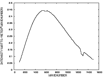
The energy content of IR radiation can be indicated by its IR spectrum which is a graph of power density as a function of frequency. Climatologists use wavenumbers instead of frequencies for convenience and a wavenumber is defined as the number of cycles per centimeter. Figure 1 is such a graph where the x axis indicates the wavenumber and the y axis indicates the power per square meter per wavenumber. The area under the curve represents the total power per square meter in the radiation.

Figure 1. IR Spectrum - No Atmosphere

The interaction of IR radiation with CO₂ is a two way street in that IR radiation can interact with unexcited CO₂ molecules and cause them to vibrate and become excited and excited CO₂ molecules can become unexcited by releasing IR radiation.

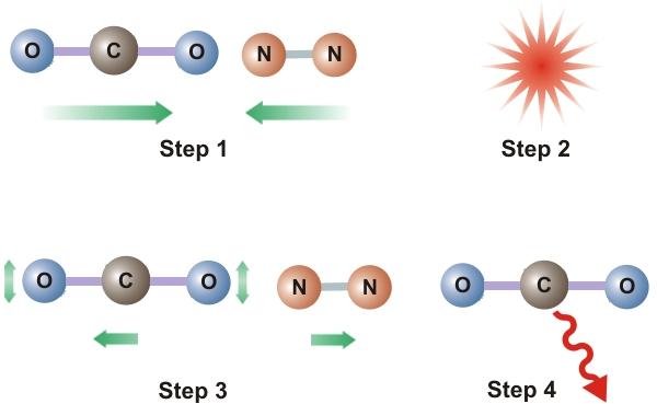
Consider now the atmosphere of our fictitious model. As depicted in Step 1 of Figure 2, N₂ and CO₂ molecules are in motion and the average speed of these molecules is related to the temperature of the stratosphere. Now imagine that CO₂ molecules are injected into the atmosphere causing the concentration of CO₂ to increase. These molecules will then collide with other molecules of either N₂ or CO₂ (Step 2) and some of the KE of these particles will be transferred to the CO₂ resulting in excited CO₂ molecules (Step 3) and a lowered stratospheric temperature. All entities, including atoms and molecules, prefer the unexcited state to the excited state. Therefore, these excited CO₂ molecules will deexcite and emit IR radiation (Step 4) which, in the rarefied stratosphere, will simply be radiated out of the stratosphere. The net result is a lower stratospheric temperature. This does not happen in the troposphere because, due to higher pressures and shorter distances between particles, any emitted radiation gets absorbed by another nearby CO₂ molecule.


Figure 2. Kinetic To IR Energy Transfer


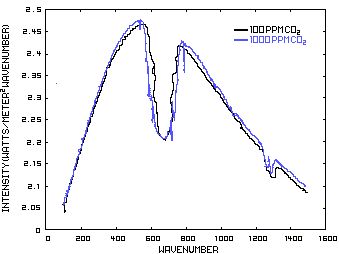
In order to discuss the second and less dominant mechanism, consider Figure 1 which shows the IR spectrum from a planet with no atmosphere and Figures 3 which shows the IR spectrums from the same planet with CO₂ levels of 100 ppm and 1000 ppm respectively. These graphs were generated from a model simulator at the website of Dr. David Archer, a professor in the Department of the Geophysical Sciences at the University of Chicago and edited to contain only the curves of interest to this discussion. As previously stated, these parameters were chosen in order to generate graphs which enable the reader to easily understand the mechanism discussed herein.
The curves of Figures 3 approximately follow the intensity curve of Figure 1 except for the missing band of energy centered at 667 cm^-1. This band is called the absorption band and is so named because it represents the IR energy that is absorbed by CO₂. IR radiation of all other wavenumbers do not react with CO₂ and thus the IR intensity at these wavenumbers is the same as that of Figure 1. These wavenumbers represent the atmospheric window which is so named because the IR energy radiates through the atmosphere unaffected by the CO₂.

Figure 3. CO₂ IR Spectrum - 100/1000 ppm

A comparison of the curves in Figure 3 shows that the absorption band at 1000 ppm is wider than that at 100 ppm because more energy has been absorbed from the IR radiation by the troposphere at a CO₂ concentration of 1000 ppm than at a concentration of 100 ppm. The energy that remains in the absorption band after the IR radiation has traveled through the troposphere is the only energy that is available to interact with the CO₂ of the stratosphere. At a CO₂ level of 100 ppm there is more energy available for this than at a level of 1000 ppm. Therefore, the stratosphere is cooler because of the higher level of CO₂ in the troposphere. Additionally, the troposphere has warmed because it has absorbed the energy that is no longer available to the stratosphere.

In concluding, this paper has explained the mechanisms which cause the troposphere to warm and the stratosphere to cool when the atmospheric level of CO₂ increases. The dominant mechanism involves the conversion of the energy of motion of the particles in the atmosphere to IR radiation which escapes to space and the second method involves the absorption of IR energy by CO₂ in the troposphere such that it is no longer available to the stratosphere. Both methods act to reduce the temperature of the stratosphere.

*It is recognized that a fictitious planet as described herein is a physical impossibility. The simplicity of this model serves to explain a concept that would otherwise be more difficult using a more complex and realistic model.

Robert J. Guercio - December 18, 2010