Search This Blog

Thursday, June 28, 2018

Mathematical and theoretical biology

From Wikipedia, the free encyclopedia

Mathematical and theoretical biology is a branch of biology which employs theoretical analysis, mathematical models and abstractions of the living organisms to investigate the principles that govern the structure, development and behavior of the systems, as opposed to experimental biology which deals with the conduction of experiments to prove and validate the scientific theories.[1] The field is sometimes called mathematical biology or biomathematics to stress the mathematical side, or theoretical biology to stress the biological side.[2] Theoretical biology focuses more on the development of theoretical principles for biology while mathematical biology focuses on the use of mathematical tools to study biological systems, even though the two terms are sometimes interchanged.

Mathematical biology aims at the mathematical representation and modeling of biological processes, using techniques and tools of applied mathematics. It has both theoretical and practical applications in biological, biomedical and biotechnology research. Describing systems in a quantitative manner means their behavior can be better simulated, and hence properties can be predicted that might not be evident to the experimenter. This requires precise mathematical models.

Mathematical biology employs many components of mathematics,[5] and has contributed to the development of new techniques.

History

Early history

Mathematics has been applied to biology since the 19th century.

Fritz Müller described the evolutionary benefits of what is now called Müllerian mimicry in 1879, in an account notable for being the first use of a mathematical argument in evolutionary ecology to show how powerful the effect of natural selection would be, unless one includes Malthus's discussion of the effects of population growth that influenced Charles Darwin: Malthus argued that growth would be "geometric" while resources (the environment's carrying capacity) could only grow arithmetically.[6]

One founding text is considered to be On Growth and Form (1917) by D'Arcy Thompson,[7] and other early pioneers include Ronald Fisher, Hans Leo Przibram, Nicolas Rashevsky and Vito Volterra.[8]

Recent growth

Interest in the field has grown rapidly from the 1960s onwards. Some reasons for this include:
  • The rapid growth of data-rich information sets, due to the genomics revolution, which are difficult to understand without the use of analytical tools
  • Recent development of mathematical tools such as chaos theory to help understand complex, non-linear mechanisms in biology
  • An increase in computing power, which facilitates calculations and simulations not previously possible
  • An increasing interest in in silico experimentation due to ethical considerations, risk, unreliability and other complications involved in human and animal research

Areas of research

Several areas of specialized research in mathematical and theoretical biology[9][10][11][12][13] as well as external links to related projects in various universities are concisely presented in the following subsections, including also a large number of appropriate validating references from a list of several thousands of published authors contributing to this field. Many of the included examples are characterised by highly complex, nonlinear, and supercomplex mechanisms, as it is being increasingly recognised that the result of such interactions may only be understood through a combination of mathematical, logical, physical/chemical, molecular and computational models.

Evolutionary biology

Ecology and evolutionary biology have traditionally been the dominant fields of mathematical biology.

Evolutionary biology has been the subject of extensive mathematical theorizing. The traditional approach in this area, which includes complications from genetics, is population genetics. Most population geneticists consider the appearance of new alleles by mutation, the appearance of new genotypes by recombination, and changes in the frequencies of existing alleles and genotypes at a small number of gene loci. When infinitesimal effects at a large number of gene loci are considered, together with the assumption of linkage equilibrium or quasi-linkage equilibrium, one derives quantitative genetics. Ronald Fisher made fundamental advances in statistics, such as analysis of variance, via his work on quantitative genetics. Another important branch of population genetics that led to the extensive development of coalescent theory is phylogenetics. Phylogenetics is an area that deals with the reconstruction and analysis of phylogenetic (evolutionary) trees and networks based on inherited characteristics[14] Traditional population genetic models deal with alleles and genotypes, and are frequently stochastic.

Many population genetics models assume that population sizes are constant. Variable population sizes, often in the absence of genetic variation, are treated by the field of population dynamics. Work in this area dates back to the 19th century, and even as far as 1798 when Thomas Malthus formulated the first principle of population dynamics, which later became known as the Malthusian growth model. The Lotka–Volterra predator-prey equations are another famous example. Population dynamics overlap with another active area of research in mathematical biology: mathematical epidemiology, the study of infectious disease affecting populations. Various models of the spread of infections have been proposed and analyzed, and provide important results that may be applied to health policy decisions.

In evolutionary game theory, developed first by John Maynard Smith and George R. Price, selection acts directly on inherited phenotypes, without genetic complications. This approach has been mathematically refined to produce the field of adaptive dynamics.

Computer models and automata theory

A monograph on this topic summarizes an extensive amount of published research in this area up to 1986,[15][16][17] including subsections in the following areas: computer modeling in biology and medicine, arterial system models, neuron models, biochemical and oscillation networks, quantum automata, quantum computers in molecular biology and genetics,[18] cancer modelling,[19] neural nets, genetic networks, abstract categories in relational biology,[20] metabolic-replication systems, category theory[21] applications in biology and medicine,[22] automata theory, cellular automata,[23] tessellation models[24][25] and complete self-reproduction, chaotic systems in organisms, relational biology and organismic theories.[26][27]

Modeling cell and molecular biology

This area has received a boost due to the growing importance of molecular biology.[12]
  • Mechanics of biological tissues[28]
  • Theoretical enzymology and enzyme kinetics
  • Cancer modelling and simulation[29][30]
  • Modelling the movement of interacting cell populations[31]
  • Mathematical modelling of scar tissue formation[32]
  • Mathematical modelling of intracellular dynamics[33][34]
  • Mathematical modelling of the cell cycle[35]
Modelling physiological systems

Molecular set theory

Molecular set theory (MST) is a mathematical formulation of the wide-sense chemical kinetics of biomolecular reactions in terms of sets of molecules and their chemical transformations represented by set-theoretical mappings between molecular sets. It was introduced by Anthony Bartholomay, and its applications were developed in mathematical biology and especially in mathematical medicine.[38] In a more general sense, MST is the theory of molecular categories defined as categories of molecular sets and their chemical transformations represented as set-theoretical mappings of molecular sets. The theory has also contributed to biostatistics and the formulation of clinical biochemistry problems in mathematical formulations of pathological, biochemical changes of interest to Physiology, Clinical Biochemistry and Medicine.[38][39]

Mathematical methods

A model of a biological system is converted into a system of equations, although the word 'model' is often used synonymously with the system of corresponding equations. The solution of the equations, by either analytical or numerical means, describes how the biological system behaves either over time or at equilibrium. There are many different types of equations and the type of behavior that can occur is dependent on both the model and the equations used. The model often makes assumptions about the system. The equations may also make assumptions about the nature of what may occur.

Simulation of mathematical biology

Computer with significant recent evolution in performance acceraretes the model simulation based on various formulas. The websites BioMath Modeler can run simulations and display charts interactively on browser.

Mathematical biophysics

The earlier stages of mathematical biology were dominated by mathematical biophysics, described as the application of mathematics in biophysics, often involving specific physical/mathematical models of biosystems and their components or compartments.

The following is a list of mathematical descriptions and their assumptions.

Deterministic processes (dynamical systems)

A fixed mapping between an initial state and a final state. Starting from an initial condition and moving forward in time, a deterministic process always generates the same trajectory, and no two trajectories cross in state space.

Stochastic processes (random dynamical systems)

A random mapping between an initial state and a final state, making the state of the system a random variable with a corresponding probability distribution.

Spatial modelling

One classic work in this area is Alan Turing's paper on morphogenesis entitled The Chemical Basis of Morphogenesis, published in 1952 in the Philosophical Transactions of the Royal Society.

Organizational biology

Theoretical approaches to biological organization aim to understand the interdependence between the parts of organisms. They emphasize the circularities that these interdependences lead to. Theoretical biologists developed several concepts to formalize this idea.

For example, abstract relational biology (ARB)[45] is concerned with the study of general, relational models of complex biological systems, usually abstracting out specific morphological, or anatomical, structures. Some of the simplest models in ARB are the Metabolic-Replication, or (M,R)--systems introduced by Robert Rosen in 1957-1958 as abstract, relational models of cellular and organismal organization.[46]

Other approaches include the notion of autopoiesis developed by Maturana and Varela, Kauffman's Work-Constraints cycles, and more recently the notion of closure of constraints.[47]

Algebraic biology

Algebraic biology (also known as symbolic systems biology) applies the algebraic methods of symbolic computation to the study of biological problems, especially in genomics, proteomics, analysis of molecular structures and study of genes.[26][48][49]

Computational neuroscience

Computational neuroscience (also known as theoretical neuroscience or mathematical neuroscience) is the theoretical study of the nervous system.

Model example: the cell cycle

The eukaryotic cell cycle is very complex and is one of the most studied topics, since its misregulation leads to cancers. It is possibly a good example of a mathematical model as it deals with simple calculus but gives valid results. Two research groups [52][53] have produced several models of the cell cycle simulating several organisms. They have recently produced a generic eukaryotic cell cycle model that can represent a particular eukaryote depending on the values of the parameters, demonstrating that the idiosyncrasies of the individual cell cycles are due to different protein concentrations and affinities, while the underlying mechanisms are conserved (Csikasz-Nagy et al., 2006).
By means of a system of ordinary differential equations these models show the change in time (dynamical system) of the protein inside a single typical cell; this type of model is called a deterministic process (whereas a model describing a statistical distribution of protein concentrations in a population of cells is called a stochastic process).

To obtain these equations an iterative series of steps must be done: first the several models and observations are combined to form a consensus diagram and the appropriate kinetic laws are chosen to write the differential equations, such as rate kinetics for stoichiometric reactions, Michaelis-Menten kinetics for enzyme substrate reactions and Goldbeter–Koshland kinetics for ultrasensitive transcription factors, afterwards the parameters of the equations (rate constants, enzyme efficiency coefficients and Michaelis constants) must be fitted to match observations; when they cannot be fitted the kinetic equation is revised and when that is not possible the wiring diagram is modified. The parameters are fitted and validated using observations of both wild type and mutants, such as protein half-life and cell size.

To fit the parameters, the differential equations must be studied. This can be done either by simulation or by analysis. In a simulation, given a starting vector (list of the values of the variables), the progression of the system is calculated by solving the equations at each time-frame in small increments.

Cell cycle bifurcation diagram.jpg

In analysis, the properties of the equations are used to investigate the behavior of the system depending of the values of the parameters and variables. A system of differential equations can be represented as a vector field, where each vector described the change (in concentration of two or more protein) determining where and how fast the trajectory (simulation) is heading. Vector fields can have several special points: a stable point, called a sink, that attracts in all directions (forcing the concentrations to be at a certain value), an unstable point, either a source or a saddle point, which repels (forcing the concentrations to change away from a certain value), and a limit cycle, a closed trajectory towards which several trajectories spiral towards (making the concentrations oscillate).

A better representation, which handles the large number of variables and parameters, is a bifurcation diagram using bifurcation theory. The presence of these special steady-state points at certain values of a parameter (e.g. mass) is represented by a point and once the parameter passes a certain value, a qualitative change occurs, called a bifurcation, in which the nature of the space changes, with profound consequences for the protein concentrations: the cell cycle has phases (partially corresponding to G1 and G2) in which mass, via a stable point, controls cyclin levels, and phases (S and M phases) in which the concentrations change independently, but once the phase has changed at a bifurcation event (Cell cycle checkpoint), the system cannot go back to the previous levels since at the current mass the vector field is profoundly different and the mass cannot be reversed back through the bifurcation event, making a checkpoint irreversible. In particular the S and M checkpoints are regulated by means of special bifurcations called a Hopf bifurcation and an infinite period bifurcation.[citation needed]

Societies and institutes

Artificial life

From Wikipedia, the free encyclopedia

Artificial life (often abbreviated ALife or A-Life) is a field of study wherein researchers examine systems related to natural life, its processes, and its evolution, through the use of simulations with computer models, robotics, and biochemistry.[1] The discipline was named by Christopher Langton, an American theoretical biologist, in 1986.[2] There are three main kinds of alife,[3] named for their approaches: soft,[4] from software; hard,[5] from hardware; and wet, from biochemistry. Artificial life researchers study traditional biology by trying to recreate aspects of biological phenomena.

A Braitenberg vehicle simulation, programmed in breve, an artificial life simulator

Overview

Artificial life studies the fundamental processes of living systems in artificial environments in order to gain a deeper understanding of the complex information processing that define such systems. These topics are broad, but often include evolutionary dynamics, emergent properties of collective systems, biomimicry, as well as related issues about the philosophy of the nature of life and the use of lifelike properties in artistic works.

Philosophy

The modeling philosophy of artificial life strongly differs from traditional modeling by studying not only "life-as-we-know-it" but also "life-as-it-might-be".[8]

A traditional model of a biological system will focus on capturing its most important parameters. In contrast, an alife modeling approach will generally seek to decipher the most simple and general principles underlying life and implement them in a simulation. The simulation then offers the possibility to analyse new and different lifelike systems.

Vladimir Georgievich Red'ko proposed to generalize this distinction to the modeling of any process, leading to the more general distinction of "processes-as-we-know-them" and "processes-as-they-could-be".[9]

At present, the commonly accepted definition of life does not consider any current alife simulations or software to be alive, and they do not constitute part of the evolutionary process of any ecosystem. However, different opinions about artificial life's potential have arisen:
  • The strong alife (cf. Strong AI) position states that "life is a process which can be abstracted away from any particular medium" (John von Neumann)[citation needed]. Notably, Tom Ray declared that his program Tierra is not simulating life in a computer but synthesizing it.[10]
  • The weak alife position denies the possibility of generating a "living process" outside of a chemical solution. Its researchers try instead to simulate life processes to understand the underlying mechanics of biological phenomena.

Organizations

Software-based ("soft")

Techniques

  • Cellular automata were used in the early days of artificial life, and are still often used for ease of scalability and parallelization. Alife and cellular automata share a closely tied history.
  • Artificial neural networks are sometimes used to model the brain of an agent. Although traditionally more of an artificial intelligence technique, neural nets can be important for simulating population dynamics of organisms that can learn. The symbiosis between learning and evolution is central to theories about the development of instincts in organisms with higher neurological complexity, as in, for instance, the Baldwin effect.

Notable simulators

This is a list of artificial life/digital organism simulators, organized by the method of creature definition.

Name Driven By Started Ended
Avida executable DNA 1993 ongoing
Neurokernel Geppetto 2014 ongoing
Creatures neural net/simulated biochemistry 1996-2001 Fandom still active to this day, some abortive attempts at new products
Critterding neural net 2005 ongoing
Darwinbots executable DNA 2003 ongoing
DigiHive executable DNA 2006 2009
DOSE executable DNA 2012 ongoing
EcoSim Fuzzy Cognitive Map 2009 ongoing
Evolve 4.0 executable DNA 1996 Prior to Nov. 2014
Framsticks executable DNA 1996 ongoing
Noble Ape neural net 1996 ongoing
OpenWorm Geppetto 2011 ongoing
Polyworld neural net 1990 ongoing
Primordial Life executable DNA 1994 2003
ScriptBots executable DNA 2010 ongoing
TechnoSphere modules 1995
Tierra executable DNA 1991 2004
3D Virtual Creature Evolution neural net 2008 NA

Program-based

Program-based simulations contain organisms with a complex DNA language, usually Turing complete. This language is more often in the form of a computer program than actual biological DNA. Assembly derivatives are the most common languages used. An organism "lives" when its code is executed, and there are usually various methods allowing self-replication. Mutations are generally implemented as random changes to the code. Use of cellular automata is common but not required. Another example could be an artificial intelligence and multi-agent system/program.

Module-based

Individual modules are added to a creature. These modules modify the creature's behaviors and characteristics either directly, by hard coding into the simulation (leg type A increases speed and metabolism), or indirectly, through the emergent interactions between a creature's modules (leg type A moves up and down with a frequency of X, which interacts with other legs to create motion). Generally these are simulators which emphasize user creation and accessibility over mutation and evolution.

Parameter-based

Organisms are generally constructed with pre-defined and fixed behaviors that are controlled by various parameters that mutate. That is, each organism contains a collection of numbers or other finite parameters. Each parameter controls one or several aspects of an organism in a well-defined way.

Neural net–based

These simulations have creatures that learn and grow using neural nets or a close derivative. Emphasis is often, although not always, more on learning than on natural selection.

Complex systems modelling

Mathematical models of complex systems are of three types: black-box (phenomenological), white-box (mechanistic, based on the first principles) and grey-box (mixtures of phenomenological and mechanistic models) [11][12]. In black-box models, the individual-based (mechanistic) mechanisms of a complex dynamic system remain hidden.

Mathematical models for complex systems

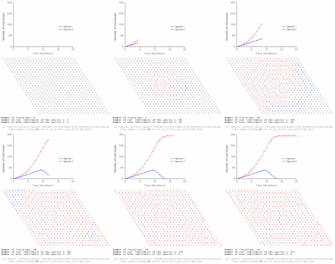
Black-box models are completely nonmechanistic. They are phenomenological and ignore a composition and internal structure of a complex system. We cannot investigate interactions of subsystems of such a non-transparent model. A white-box model of complex dynamic system has ‘transparent walls’ and directly shows underlying mechanisms. All events at micro-, meso- and macro-levels of a dynamic system are directly visible at all stages of its white-box model evolution. In most cases mathematical modelers use the heavy black-box mathematical methods, which cannot produce mechanistic models of complex dynamic systems. Grey-box models are intermediate and combine black-box and white-box approaches.

Logical deterministic individual-based cellular automata model of single species population growth

Creation of a white-box model of complex system is associated with the problem of the necessity of an a priori basic knowledge of the modeling subject. The deterministic logical cellular automata are necessary but not sufficient condition of a white-box model. The second necessary prerequisite of a white-box model is the presence of the physical ontology of the object under study. The white-box modeling represents an automatic hyper-logical inference from the first principles because it is completely based on the deterministic logic and axiomatic theory of the subject. The purpose of the white-box modeling is to derive from the basic axioms a more detailed, more concrete mechanistic knowledge about the dynamics of the object under study. The necessity to formulate an intrinsic axiomatic system of the subject before creating its white-box model distinguishes the cellular automata models of white-box type from cellular automata models based on arbitrary logical rules. If cellular automata rules have not been formulated from the first principles of the subject, then such a model may have a weak relevance to the real problem [12].

Logical deterministic individual-based cellular automata model of interspecific competition for a single limited resource

Hardware-based ("hard")

Hardware-based artificial life mainly consist of robots, that is, automatically guided machines able to do tasks on their own.

Biochemical-based ("wet")

Biochemical-based life is studied in the field of synthetic biology. It involves e.g. the creation of synthetic DNA. The term "wet" is an extension of the term "wetware".

Open problems

How does life arise from the nonliving?[13][14]
  • Generate a molecular proto-organism in vitro.
  • Achieve the transition to life in an artificial chemistry in silico.
  • Determine whether fundamentally novel living organizations can exist.
  • Simulate a unicellular organism over its entire life cycle.
  • Explain how rules and symbols are generated from physical dynamics in living systems.
What are the potentials and limits of living systems?
  • Determine what is inevitable in the open-ended evolution of life.
  • Determine minimal conditions for evolutionary transitions from specific to generic response systems.
  • Create a formal framework for synthesizing dynamical hierarchies at all scales.
  • Determine the predictability of evolutionary consequences of manipulating organisms and ecosystems.
  • Develop a theory of information processing, information flow, and information generation for evolving systems.
How is life related to mind, machines, and culture?
  • Demonstrate the emergence of intelligence and mind in an artificial living system.
  • Evaluate the influence of machines on the next major evolutionary transition of life.
  • Provide a quantitative model of the interplay between cultural and biological evolution.
  • Establish ethical principles for artificial life.

Related subjects

  1. Artificial intelligence has traditionally used a top down approach, while alife generally works from the bottom up.[15]
  2. Artificial chemistry started as a method within the alife community to abstract the processes of chemical reactions.
  3. Evolutionary algorithms are a practical application of the weak alife principle applied to optimization problems. Many optimization algorithms have been crafted which borrow from or closely mirror alife techniques. The primary difference lies in explicitly defining the fitness of an agent by its ability to solve a problem, instead of its ability to find food, reproduce, or avoid death.[citation needed] The following is a list of evolutionary algorithms closely related to and used in alife:
  4. Multi-agent system – A multi-agent system is a computerized system composed of multiple interacting intelligent agents within an environment.
  5. Evolutionary art uses techniques and methods from artificial life to create new forms of art.
  6. Evolutionary music uses similar techniques, but applied to music instead of visual art.
  7. Abiogenesis and the origin of life sometimes employ alife methodologies as well.

Criticism

Alife has had a controversial history. John Maynard Smith criticized certain artificial life work in 1994 as "fact-free science".[16]

Fuzzy logic

From Wikipedia, the free encyclopedia

Fuzzy logic is a form of many-valued logic in which the truth values of variables may be any real number between 0 and 1. It is employed to handle the concept of partial truth, where the truth value may range between completely true and completely false.[1] By contrast, in Boolean logic, the truth values of variables may only be the integer values 0 or 1.

The term fuzzy logic was introduced with the 1965 proposal of fuzzy set theory by Lotfi Zadeh.[2][3] Fuzzy logic had however been studied since the 1920s, as infinite-valued logic—notably by Łukasiewicz and Tarski.[4]

Fuzzy logic has been applied to many fields, from control theory to artificial intelligence.

Overview

Classical logic only permits conclusions which are either true or false. However, there are also propositions with variable answers, such as one might find when asking a group of people to identify a color. In such instances, the truth appears as the result of reasoning from inexact or partial knowledge in which the sampled answers are mapped on a spectrum.[citation needed]

Both degrees of truth and probabilities range between 0 and 1 and hence may seem similar at first, but fuzzy logic uses degrees of truth as a mathematical model of vagueness, while probability is a mathematical model of ignorance.[citation needed]

Applying truth values

A basic application might characterize various sub-ranges of a continuous variable. For instance, a temperature measurement for anti-lock brakes might have several separate membership functions defining particular temperature ranges needed to control the brakes properly. Each function maps the same temperature value to a truth value in the 0 to 1 range. These truth values can then be used to determine how the brakes should be controlled.[citation needed]

Linguistic variables

While variables in mathematics usually take numerical values, in fuzzy logic applications, non-numeric values are often used to facilitate the expression of rules and facts.[5]

A linguistic variable such as age may accept values such as young and its antonym old. Because natural languages do not always contain enough value terms to express a fuzzy value scale, it is common practice to modify linguistic values with adjectives or adverbs. For example, we can use the hedges rather and somewhat to construct the additional values rather old or somewhat young.

Fuzzification operations can map mathematical input values into fuzzy membership functions. And the opposite de-fuzzifying operations can be used to map a fuzzy output membership functions into a "crisp" output value that can be then used for decision or control purposes.

Process

  1. Fuzzify all input values into fuzzy membership functions.
  2. Execute all applicable rules in the rulebase to compute the fuzzy output functions.
  3. De-fuzzify the fuzzy output functions to get "crisp" output values.

Fuzzification


Fuzzy logic temperature

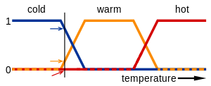
In this image, the meanings of the expressions cold, warm, and hot are represented by functions mapping a temperature scale. A point on that scale has three "truth values"—one for each of the three functions. The vertical line in the image represents a particular temperature that the three arrows (truth values) gauge. Since the red arrow points to zero, this temperature may be interpreted as "not hot". The orange arrow (pointing at 0.2) may describe it as "slightly warm" and the blue arrow (pointing at 0.8) "fairly cold".

Fuzzy sets are often defined as triangle or trapezoid-shaped curves, as each value will have a slope where the value is increasing, a peak where the value is equal to 1 (which can have a length of 0 or greater) and a slope where the value is decreasing.[citation needed] They can also be defined using a sigmoid function.[6] One common case is the standard logistic function defined as
{\displaystyle S(x)={\frac {1}{1+e^{-x}}}}
which has the following symmetry property
{\displaystyle S(x)+S(-x)=1}
From this it follows that

{\displaystyle (S(x)+S(-x))\cdot (S(y)+S(-y))\cdot (S(z)+S(-z))=1}

Fuzzy logic operators

Fuzzy logic works with membership values in a way that mimics Boolean logic.[citation needed]

To this end, replacements for basic operators AND, OR, NOT must be available. There are several ways to this. A common replacement is called the Zadeh operators:

Boolean Fuzzy
AND(x,y) MIN(x,y)
OR(x,y) MAX(x,y)
NOT(x) 1 – x

For TRUE/1 and FALSE/0, the fuzzy expressions produce the same result as the Boolean expressions.

There are also other operators, more linguistic in nature, called hedges that can be applied. These are generally adverbs such as very, or somewhat, which modify the meaning of a set using a mathematical formula.

However, an arbitrary choice table does not always define a fuzzy logic function. In the paper,[7] a criterion has been formulated to recognize whether a given choice table defines a fuzzy logic function and a simple algorithm of fuzzy logic function synthesis has been proposed based on introduced concepts of constituents of minimum and maximum. A fuzzy logic function represents a disjunction of constituents of minimum, where a constituent of minimum is a conjunction of variables of the current area greater than or equal to the function value in this area (to the right of the function value in the inequality, including the function value).

Another set of AND/OR operators is based on multiplication

x AND y = x*y
x OR y = 1-(1-x)*(1-y) = x+y-x*y
 
1-(1-x)*(1-y) comes from this:

x OR y = NOT( AND( NOT(x), NOT(y) ) )
x OR y = NOT( AND(1-x, 1-y) )
x OR y = NOT( (1-x)*(1-y) )
x OR y = 1-(1-x)*(1-y)

IF-THEN rules

IF-THEN rules map input or computed truth values to desired output truth values. Example:

IF temperature IS very cold THEN fan_speed is stopped
IF temperature IS cold THEN fan_speed is slow
IF temperature IS warm THEN fan_speed is moderate
IF temperature IS hot THEN fan_speed is high

Given a certain temperature, the fuzzy variable hot has a certain truth value, which is copied to the high variable.

Should an output variable occur in several THEN parts, then the values from the respective IF parts are combined using the OR operator.

Defuzzification

The goal is to get a continuous variable from fuzzy truth values.[citation needed]
This would be easy if the output truth values were exactly those obtained from fuzzification of a given number. Since, however, all output truth values are computed independently, in most cases they do not represent such a set of numbers.[citation needed] One has then to decide for a number that matches best the "intention" encoded in the truth value. For example, for several truth values of fan_speed, an actual speed must be found that best fits the computed truth values of the variables 'slow', 'medium' and so on.[citation needed]

There is no single algorithm for this purpose.

A common algorithm is
  1. For each truth value, cut the membership function at this value
  2. Combine the resulting curves using the OR operator
  3. Find the center-of-weight of the area under the curve
  4. The x position of this center is then the final output.

Forming a consensus of inputs and fuzzy rules

Since the fuzzy system output is a consensus of all of the inputs and all of the rules, fuzzy logic systems can be well behaved when input values are not available or are not trustworthy. Weightings can be optionally added to each rule in the rulebase and weightings can be used to regulate the degree to which a rule affects the output values. These rule weightings can be based upon the priority, reliability or consistency of each rule. These rule weightings may be static or can be changed dynamically, even based upon the output from other rules.

Early applications

Many of the early successful applications of fuzzy logic were implemented in Japan. The first notable application was on the subway train in Sendai, in which fuzzy logic was able to improve the economy, comfort, and precision of the ride.[8] It has also been used in recognition of hand written symbols in Sony pocket computers, flight aid for helicopters, controlling of subway systems in order to improve driving comfort, precision of halting, and power economy, improved fuel consumption for automobiles, single-button control for washing machines, automatic motor control for vacuum cleaners with recognition of surface condition and degree of soiling, and prediction systems for early recognition of earthquakes through the Institute of Seismology Bureau of Meteorology, Japan.[9]

Logical analysis

In mathematical logic, there are several formal systems of "fuzzy logic", most of which are in the family of t-norm fuzzy logics.

Propositional fuzzy logics

The most important propositional fuzzy logics are:
  • Monoidal t-norm-based propositional fuzzy logic MTL is an axiomatization of logic where conjunction is defined by a left continuous t-norm and implication is defined as the residuum of the t-norm. Its models correspond to MTL-algebras that are pre-linear commutative bounded integral residuated lattices.
  • Basic propositional fuzzy logic BL is an extension of MTL logic where conjunction is defined by a continuous t-norm, and implication is also defined as the residuum of the t-norm. Its models correspond to BL-algebras.
  • Łukasiewicz fuzzy logic is the extension of basic fuzzy logic BL where standard conjunction is the Łukasiewicz t-norm. It has the axioms of basic fuzzy logic plus an axiom of double negation, and its models correspond to MV-algebras.
  • Gödel fuzzy logic is the extension of basic fuzzy logic BL where conjunction is Gödel t-norm. It has the axioms of BL plus an axiom of idempotence of conjunction, and its models are called G-algebras.
  • Product fuzzy logic is the extension of basic fuzzy logic BL where conjunction is product t-norm. It has the axioms of BL plus another axiom for cancellativity of conjunction, and its models are called product algebras.
  • Fuzzy logic with evaluated syntax (sometimes also called Pavelka's logic), denoted by EVŁ, is a further generalization of mathematical fuzzy logic. While the above kinds of fuzzy logic have traditional syntax and many-valued semantics, in EVŁ is evaluated also syntax. This means that each formula has an evaluation. Axiomatization of EVŁ stems from Łukasziewicz fuzzy logic. A generalization of classical Gödel completeness theorem is provable in EVŁ.

Predicate fuzzy logics

These extend the above-mentioned fuzzy logics by adding universal and existential quantifiers in a manner similar to the way that predicate logic is created from propositional logic. The semantics of the universal (resp. existential) quantifier in t-norm fuzzy logics is the infimum (resp. supremum) of the truth degrees of the instances of the quantified subformula.

Decidability issues for fuzzy logic

The notions of a "decidable subset" and "recursively enumerable subset" are basic ones for classical mathematics and classical logic. Thus the question of a suitable extension of them to fuzzy set theory is a crucial one. A first proposal in such a direction was made by E.S. Santos by the notions of fuzzy Turing machine, Markov normal fuzzy algorithm and fuzzy program (see Santos 1970). Successively, L. Biacino and G. Gerla argued that the proposed definitions are rather questionable. For example, in [10] one shows that the fuzzy Turing machines are not adequate for fuzzy language theory since there are natural fuzzy languages intuitively computable that cannot be recognized by a fuzzy Turing Machine. Then, they proposed the following definitions. Denote by Ü the set of rational numbers in [0,1]. Then a fuzzy subset s : S \rightarrow [0,1] of a set S is recursively enumerable if a recursive map h : S×N \rightarrow Ü exists such that, for every x in S, the function h(x,n) is increasing with respect to n and s(x) = lim h(x,n). We say that s is decidable if both s and its complement –s are recursively enumerable. An extension of such a theory to the general case of the L-subsets is possible (see Gerla 2006). The proposed definitions are well related with fuzzy logic. Indeed, the following theorem holds true (provided that the deduction apparatus of the considered fuzzy logic satisfies some obvious effectiveness property).

Any "axiomatizable" fuzzy theory is recursively enumerable. In particular, the fuzzy set of logically true formulas is recursively enumerable in spite of the fact that the crisp set of valid formulas is not recursively enumerable, in general. Moreover, any axiomatizable and complete theory is decidable.

It is an open question to give supports for a "Church thesis" for fuzzy mathematics, the proposed notion of recursive enumerability for fuzzy subsets is the adequate one. In order to solve this, an extension of the notions of fuzzy grammar and fuzzy Turing machine are necessary. Another open question is to start from this notion to find an extension of Gödel's theorems to fuzzy logic.

Fuzzy databases

Once fuzzy relations are defined, it is possible to develop fuzzy relational databases. The first fuzzy relational database, FRDB, appeared in Maria Zemankova's dissertation (1983). Later, some other models arose like the Buckles-Petry model, the Prade-Testemale Model, the Umano-Fukami model or the GEFRED model by J.M. Medina, M.A. Vila et al.

Fuzzy querying languages have been defined, such as the SQLf by P. Bosc et al. and the FSQL by J. Galindo et al. These languages define some structures in order to include fuzzy aspects in the SQL statements, like fuzzy conditions, fuzzy comparators, fuzzy constants, fuzzy constraints, fuzzy thresholds, linguistic labels etc.

Comparison to probability

Fuzzy logic and probability address different forms of uncertainty. While both fuzzy logic and probability theory can represent degrees of certain kinds of subjective belief, fuzzy set theory uses the concept of fuzzy set membership, i.e., how much an observation is within a vaguely defined set, and probability theory uses the concept of subjective probability, i.e., likelihood of some event or condition. The concept of fuzzy sets was developed in the mid-twentieth century at Berkeley [11] as a response to the lacking of probability theory for jointly modelling uncertainty and vagueness.[12]

Bart Kosko claims in Fuzziness vs. Probability that probability theory is a subtheory of fuzzy logic, as questions of degrees of belief in mutually-exclusive set membership in probability theory can be represented as certain cases of non-mutually-exclusive graded membership in fuzzy theory. In that context, he also derives Bayes' theorem from the concept of fuzzy subsethood. Lotfi A. Zadeh argues that fuzzy logic is different in character from probability, and is not a replacement for it. He fuzzified probability to fuzzy probability and also generalized it to possibility theory.

More generally, fuzzy logic is one of many different extensions to classical logic intended to deal with issues of uncertainty outside of the scope of classical logic, the inapplicability of probability theory in many domains, and the paradoxes of Dempster-Shafer theory.

Relation to ecorithms

Computational theorist Leslie Valiant uses the term ecorithms to describe how many less exact systems and techniques like fuzzy logic (and "less robust" logic) can be applied to learning algorithms. Valiant essentially redefines machine learning as evolutionary. In general use, ecorithms are algorithms that learn from their more complex environments (hence eco-) to generalize, approximate and simplify solution logic. Like fuzzy logic, they are methods used to overcome continuous variables or systems too complex to completely enumerate or understand discretely or exactly. [14] Ecorithms and fuzzy logic also have the common property of dealing with possibilities more than probabilities, although feedback and feed forward, basically stochastic weights, are a feature of both when dealing with, for example, dynamical systems.

Compensatory fuzzy logic

Compensatory fuzzy logic (CFL) is a branch of fuzzy logic with modified rules for conjunction and disjunction. When the truth value of one component of a conjunction or disjunction is increased or decreased, the other component is decreased or increased to compensate. This increase or decrease in truth value may be offset by the increase or decrease in another component. An offset may be blocked when certain thresholds are met. Proponents claim that CFL allows for better computational semantic behaviors and mimic natural language.

Compensatory Fuzzy Logic consists of four continuous operators: conjunction (c); disjunction (d); fuzzy strict order (or); and negation (n). The conjunction is the geometric mean and its dual as conjunctive and disjunctive operators.[17]

IEEE STANDARD 1855–2016 – IEEE Standard for Fuzzy Markup Language

The IEEE 1855, the IEEE STANDARD 1855–2016, is about a specification language named Fuzzy Markup Language (FML)[18] developed by the IEEE Standards Association. FML allows modelling a fuzzy logic system in a human-readable and hardware independent way. FML is based on eXtensible Markup Language (XML). The designers of fuzzy systems with FML have a unified and high-level methodology for describing interoperable fuzzy systems. IEEE STANDARD 1855–2016 uses the W3C XML Schema definition language to define the syntax and semantics of the FML programs.

Prior to the introduction of FML, fuzzy logic practitioners could exchange information about their fuzzy algorithms by  adding to their software functions the ability to read, correctly parse, and store the results of their work in a  form compatible with the Fuzzy Control Language (FCL) described and specified by Part 7 of IEC 61131.[19][20]

Lie point symmetry

From Wikipedia, the free encyclopedia https://en.wikipedia.org/wiki/Lie_point_symmetry     ...