A Medley of Potpourri

Sunday, May 8, 2022

History of children in the military

From Wikipedia, the free encyclopedia

https://en.wikipedia.org/wiki/History_of_children_in_the_military

A Chinese Nationalist soldier, age 10, from the Chinese Army in India waiting to board a plane in Burma, May 1944

Child soldiers
Part of a series on
Main articles
Child soldiers History Piracy Impact Rehabilitation and reintegration
Issues
Abduction Sexual abuse Trafficking Prostitution Post-traumatic stress disorder
Instances (examples)
World War II Africa Central African Republic Democratic Republic of Congo India Myanmar Palestine Sierra Leone Somalia Sri Lanka
Legal aspects
Paris Principles Convention on the Rights of the Child Optional protocol
Movement to end the use of child soldiers
Red Hand Day

Children in the military are children (defined by the Convention on the Rights of the Child as persons under the age of 18) who are associated with military organizations, such as state armed forces and non-state armed groups. Throughout history and in many cultures, children have been involved in military campaigns. For example, thousands of children participated on all sides of the First World War and the Second World War. Children may be trained and used for combat, assigned to support roles such as porters or messengers, or used for tactical advantage as human shields or for political advantage in propaganda.

Children are easy targets for military recruitment due to their greater susceptibility to influence compared to adults. Some children are recruited by force while others choose to join up, often to escape poverty or because they expect military life to offer a rite of passage to maturity.

Pre-20th century

Mexico honors its cadets who died in the Battle of Chapultepec (1847).

Throughout history and in many cultures, children have been extensively involved in military campaigns.

The earliest mentions of minors being involved in wars come from antiquity. It was customary for youths in the Mediterranean basin to serve as aides, charioteers and armor bearers to adult warriors. Examples of this practice can be found in the Bible, such as David's service to King Saul, in Hittite and ancient Egyptian art, and in ancient Greek mythology (such as the story of Hercules and Hylas), philosophy and literature. In a practice dating back to antiquity, children were routinely taken on a campaign, together with the rest of a military man's family, as part of the baggage.

The Roman Empire made use of youths in war, though it was understood that it was unwise and cruel to use children in war, and Plutarch implies that regulations required youths to be at least sixteen years of age.^{[citation needed]} Despite this, several Roman legionaries were known to have enlisted children aged 14 in the Imperial Roman army, such as Quintus Postunius Solus who completed 21 years of service in Legio XX Valeria Victrix, and Caecilius Donatus who served 26 years in the Legio XX and died shortly before his honorable discharge.

In medieval Europe young boys from about twelve years of age were used as military aides ("squires"), though in theory, their role in actual combat was limited. The so-called Children's Crusade in 1212 recruited thousands of children as untrained soldiers under the assumption that divine power would enable them to conquer the enemy, although none of the children entered combat. According to the legend, they were instead sold into slavery. While most scholars no longer believe that the Children's Crusade consisted solely, or even mostly, of children, it nonetheless exemplifies an era in which entire families took part in a war effort.

Lemuel Cook (1759-1866) served 1775–1784 in the American Revolutionary War
Samuel Downing (b. 1762) served in the American Revolution
Adam Link (1762-1864) served in the American Revolution
Daniel Waldo (1762-1864) served 1778–1779 in the American Revolution
William Hutchings (b. 1764) served in the American Revolution
Alexander Milliner (b. 1759 or 1770) served in the American Revolution

A powder monkey Aspinwall Fuller on a Union vessel, USS New Hampshire American Civil War, 1864

Young boys often took part in battles during early modern warfare. When Napoleon was faced with invasion by a massive Allied force in 1814 he conscripted many teenagers for his armies. Orphans of the Imperial Guard fought in the Netherlands with Marshal MacDonald and were between the ages of 14 and 17. Many of the conscripts who reported to the ranks in 1814 were referred to as Marie Louises after the Empress Marie Louise of France; they were also known as "The Infants of the Emperor". These soldiers were in their mid-teens. One of their more visible roles was as the ubiquitous "drummer boy".

During the age of sail, young boys formed part of the crew of British Royal Navy ships and were responsible for many essential tasks including bringing powder and shot from the ship's magazine to the gun crews. These children were called "powder monkeys."

Drummer boy John Clem during the American Civil War.

During the American Civil War a young boy, Bugler John Cook, served in the US Army at the age of 15 and received the Medal of Honor for his acts during the Battle of Antietam, the bloodiest day in American history. Several other minors, including 11-year-old Willie Johnston, have also received the Medal of Honor.

By a law signed by Nicholas I of Russia in 1827 a disproportionate number of Jewish boys, known as the cantonists, were forced into military training establishments to serve in the army. The 25-year conscription term officially commenced at the age of 18, but boys as young as eight were routinely taken to fulfill the quota.

In the final stages of the Paraguayan War, children fought in the Battle of Acosta Ñu against the Allied forces of Brazil, Argentina and Uruguay. The day is commemorated as a national holiday in Paraguay.

During the Boshin War, the pro-shōgun Aizu Domain formed the Byakkotai (白虎隊, "White Tiger Force"), which was made up of the 16 to 17-year-old sons of Aizu samurai. During the Battle of Bonari Pass and the Battle of Aizu, they fought the Satcho forces who supported the Imperial cause. A detached unit of Byakkotai was cut off from the rest of the unit and retreated to Iimori Hill, which overlooked Aizu-Wakamatsu Castle. From there, they saw what they thought was the castle on fire. 20 of the detached unit committed seppuku while one was unsuccessful. He was saved by a local peasant.

World War I

Momčilo Gavrić and another soldier reporting to major Stevan Tucović, 1916.

The youngest known soldier of World War I was Momčilo Gavrić, who joined the 6th Artillery Division of the Serbian Army at the age of 8, after Austro-Hungarian troops in August 1914 killed his parents, grandmother, and seven of his siblings.

In the West, boys as young as 12 were caught up in the overwhelming tide of patriotism and in huge numbers enlisted for active service. Others enlisted to avoid harsh and dreary lives. Typically many were able to pass themselves off as older men, such as George Thomas Paget, who at 17 joined a Bantam battalion in the Welsh Regiment. In the Gallipoli campaign, otherwise known as "Çanakkale", children as young as 15 fought in the trenches. 120 children fought in the "15'liler" or "The 15s" company, with no known survivors.

Spanish Civil War

Many child soldiers fought in the Spanish Civil War:

The centuria was an untrained mob composed mostly of boys in their teens. Here and there in the militia you came across children as young as eleven or twelve, typically refugees from Fascist territory who had been enlisted as militiamen as the easiest way of providing for them. As a rule, they were employed on light work in the rear, but sometimes they managed to worm their way to the front line, where they were a public menace. I remember one little brute throwing a hand-grenade into the dug-out fire 'for a joke'. At Monte Pocero I do not think there was anyone younger than fifteen, but the average age must have been well under twenty. Boys of this age ought never to be used in the front line because they cannot stand the lack of sleep which is inseparable from trench warfare. At the beginning, it was almost impossible to keep our position properly guarded at night. The wretched children of my section could only be roused by dragging them out of their dug-outs feet foremost, and as soon as your back was turned they left their posts and slipped into shelter; or they would even, in spite of the frightful cold, lean up against the wall of the trench and fall fast asleep.
— George Orwell

World War II

Child soldiers during the Warsaw Uprising

In World War II children under the age of 18 were widely used by all sides in formal and informal military roles. Children were readily indoctrinated into the prevailing ideology of the warring parties, quickly trained, and often sent to the front line; many were wounded or killed. The lack of a legal definition of a child, combined with the absence of a system for verifying the ages of prospective child recruits, contributed to the extensive use of children in the war.

After World War II: Historical examples by region

These are historical examples. For instances of children in the military today, see Children in the military.

Africa

Algeria

During the Algerian civil war (1991–2002) children were recruited frequently by Islamist armed groups fighting the government. A government-allied militia—the Legitimate Defence Groups (LDG)—also used children, according to some reports. Although the rules for joining the LDG were the same as the army, in which only adults were recruited (by conscription) the LDG applied no safeguards to ensure that children could not join up. The extent of child recruitment during the war remains unknown.

Burundi

Children were kidnapped and used extensively during the civil war of 1993–2005. In 2004 hundreds of child soldiers were in the Forces Nationales pour la Libération (FNL), an armed rebel, Hutu group. Children between the ages of 10 and 16 were also conscripted by the Burundese military.

After the Arusha peace accord of 2001 and the Pretoria agreement of 2003 eventually brought the conflict to an end in 2005, the new constitution committed to not using children in direct combat. The parties to the conflict no longer recruited children in large numbers, but many remained active in the FNL, which had denounced the peace accord.

By 2006, a reintegration program organized by UNICEF had led to the release of 3,000 children from the military and armed groups. According to Child Soldiers International:

The majority of those [children] who took part in the program returned to farm and fish in their local communities, but nearly 600 returned to school. Some 1,800 former child soldiers received occupational training. Health care was provided for those with special needs and psychosocial support was provided through individual and group meetings.

As of 2017, Burundi no longer appears on the UN list of countries where children are used in hostilities.

Chad

Between 2007 and 2012, children were used extensively by the Chadian military as participants in armed conflict. They were also integrated into various rebel forces, including the United Front for Democratic Change (Front Uni pour le Changement, FUC), local self-defense forces known as Tora Boro militias, and two Sudanese rebel movements operating in Chad: the Justice and Equality Movement (JEM) and the G-19 faction of the Sudanese Liberation Army (SLA). After the government signed an action plan with the United Nations, children were released from service and were no longer recruited. By 2014, Chad had been removed from the UN list of countries that use child soldiers in war.

Côte d'Ivoire

During Côte d'Ivoire's civil war of 2002–2004, "children were recruited, often forcibly, by both sides", and were also abducted by armed groups fighting the civil war in Liberia between 1999 and 2003. The Patriotic Youth – armed groups that included children in large numbers – received the active support of the government. Thousands of children saw membership of an armed group on either side of the war as a way to earn a living, although they were often unpaid, having to acquire money through extortion or begging. They were provided with automatic weapons, and girls were frequently abducted as sex slaves.

Attempts to reach a peace agreement repeatedly failed, and although after 2006 children were gradually released from military groups, approximately 2,000 children remained. After President Laurent Gbagbo refused to recognise the 2010 election result, fighting flared up again and child recruitment increased. Under the new government, however, the UN brokered an Action Plan that included the release of all children and, in 2015, the UN reported that children were no longer recruited in the country.

Eritrea

During its 30-year war for independence with Ethiopia (1961–1991) the Eritrean People's Liberation Front was "widely acknowledged" to have used children extensively as soldiers, according to the Coalition to Stop the Use of Child Soldiers (now Child Soldiers International). Once independence had been won, the Eritrean armed forces recruited and used children again during the two-year border war with Ethiopia in 1998. There were many reports of child recruitment and use (including conscription from age 15), but there is little information today about the extent of the practice, which is due in part to the absence of effective birth registration and age-verification system at the time.

The UN reported in 2002 that children were no longer being used systematically by the Eritrean armed forces, and the government acceded to the Optional Protocol on the involvement of children in armed conflict in 2005. Child recruitment continued, however; Human Rights Concern Eritrea reported in 2013 that all schoolchildren in 11th grade (approx. age 16) were made to spend the year at a military training camp, after which they were routinely recruited into the armed forces.

Ethiopia

According to the Coalition to Stop the Use of Child Soldiers in 2001 there were "credible reports" that the Ethiopian armed forces used thousands of children in its two-year border war with Eritrea between 1998 and 2000:

Testimonies of former child soldiers, NGOs and journalists provide evidence of child deployment on the front lines and in massive waves across mine fields... Recruitment reportedly focused on Oromos and Somalis... and on grades 9 to 12 of secondary schools.

Children were also forcibly recruited in groups from public places. The lack of a functioning birth registration system has made it difficult to estimate the number of children affected, but it is clear that the use of children was widespread; for example, most Ethiopian prisoners of war in one large prisoner of war camp in Eritrea were estimated to be aged 14–18.

The main opposition group in the 1990s, the Oromo Liberation Front, also systematically recruited children, including by force.

In 2008 it was reported that children were no longer used for military purposes in Ethiopia, and in 2014 the government ratified the Optional Protocol on the involvement of children in armed conflict.

Liberia

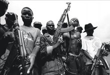
Unidentified rebel fighters during the Second Liberian Civil War, 1999–2003.

In Liberia's civil wars (1989–1995, 1999–2003) all factions abducted children for direct combat, forced labour, and sexual slavery. It was the common practice of commanders to give children drugs and threaten them with execution in order to enhance their obedience; for example, soldiers were frequently given valium before a battle, known as "bubbles" or "10-10". Children were often persuaded or forced to commit grave human rights violations against civilians, including rape, torture, and the abduction of other children for military use. Children as young as 10 were used in direct combat.

United Nations disarmament, demobilisation and reintegration programs repeatedly failed when children quitted them, often to return to their former military unit, and after fighters rioted in protest at the absence of a financial reward for being disarmed. A chronic lack of resources for reintegration also prompted child soldiers to enrol in other armed groups as a means of gainful employment. By 2004 more than 20,000 children needed to be demobilised and reunited with their communities. However, by October 2004 10,000 children had been released from their military units and were part of reintegration programs.

By 2006 children were no longer being used by any military groups in the country, although armed groups from Côte d'Ivoire and Guinea continued to abduct Liberian children. As of 2018, children were no longer being used for military purposes in Liberia, and its armed forces were recruiting only adults over the age of 18.

The use of child soldiers in Liberia was epitomised by The Small Boys Unit, established by Liberian President Charles Taylor. The boys were not provided with sustenance, but were expected to engage in "snake patrol", looting surrounding villages. Taylor and others were later tried before the Special Court for Sierra Leone because of his involvement in recruiting child soldiers.

Rwanda

Displaced children in the Democratic Republic of the Congo at risk of recruitment by Rwandese armed groups and local armed bandits.

An estimated 20,000 children took part in hostilities during the 1990s, including the 1994 Rwanda genocide when many children were involved in committing atrocities. 5,000 children were in the national army, while others, including many street children, joined or were made to join armed groups. After the genocide, 4,500 children were detained on suspicion of participating in atrocities, and were incarcerated for several years without charge or trial; some were sent to the Gitagata Re-Education Centre for males below 14 years of age. In the late 1990s, children were widely recruited again, often by force, to fight in the Democratic Republic of the Congo (DRC).

Initial demobilisation and reintegration programmes failed after many schools banned former child soldiers and a high rate of unemployment rendered them vulnerable to re-recruitment by militia groups. In 2003, as the Rwandan military presence in the DRC reduced, so did the demand for child soldiers. The government introduced new legislation to raise the minimum enlistment age 18 and the armed forces stopped recruiting children. Nonetheless, armed groups continued to do so, albeit to a reduced extent, for their operations in the DRC.

Sierra Leone

During the Sierra Leone Civil War (1991–2002) thousands of children were recruited by government armed forces and non-government armed groups, particularly the anti-government Revolutionary United Front (RUF) and the Armed Forces Revolutionary Council (AFRC), and the pro-government Civil Defence Forces (CDF).

Children were often forcibly recruited, given drugs and used to commit atrocities. Thousands of girls were also recruited as soldiers and often subjected to sexual exploitation. Many of the children were survivors of attacks on villages, which were routinely ordered to hand over their children to armed groups. By 2001, an estimated 10,000 children were being used for military purposes by government armed forces and various armed groups, particularly the RUF.

After 2002, when the war was declared over, an extensive United Nations disarmament, demobilisation and reintegration programme reunited most former child soldiers with their communities, although it drew criticism for neglecting the needs of women and girls.

In June 2007 the Special Court for Sierra Leone found three men from the rebel Armed Forces Revolutionary Council (AFRC) guilty of war crimes, crimes against humanity, and other serious violations of international humanitarian law, including the recruitment of children under the age of 15 years into the armed forces. With this the Special Court became the first ever UN-backed tribunal to secure a conviction for the military conscription of children.

As of 2018, children were no longer being used for military purposes in Sierra Leone, and its armed forces were recruiting only adults over the age of 18.

In his book A Long Way Gone: Memoirs of a Child Soldier, Ishmael Beah chronicles his life during the conflict in Sierra Leone. In Armies of the Young: Child Soldiers in War and Terrorism anthropologist David M. Rosen discusses the murders, rapes, tortures, and thousands of amputations committed by the RUF Small Boys Unit. The film Blood Diamond is set during the civil war. The issue is also explored in the Bones episode, The Survivor In The Soap.

Uganda

David Livingstone speaks about his experiences as a child soldier with the Lord's Resistance Army in Uganda.

Over a period of twenty years the rebel Lord's Resistance Army (LRA) has abducted more than 30,000 boys and girls as soldiers or sex slaves. Joseph Kony began the Lord's Resistance Army (LRA) in 1987, originally to protect northern Ugandans from the 1986 military coup by the People's National Resistance Army. Stating that he "received messages from God" Kony began attacking his own people, the Acholi, to establish a new theocratic government in Uganda based on the principles of the "Ten Commandments of God". This attempt by the LRA to gain control of the Ugandan government via roaming armies used boy- as well as girl-children as soldiers, such as Grace Akallo.

The LRA expansion into South Sudan, the Central African Republic and the Democratic Republic of Congo has used large numbers of children as active combatants and participants in extreme violence. On the 21 October 2008 an appeal by the UN Security Council was made asking for the LRA to cease all military action in the DRC immediately. On 14 June 2002 Uganda deposited its instrument of ratification of the Rome Statute, and on 16 December 2003 the Government of Uganda referred the situation concerning northern Uganda to the prosecutor of the International Criminal Court (ICC). The ICC investigated the situation and on 14 October 2005 issued indictments against Lord's Resistance Army leader Joseph Kony and four other commanders for war crimes: Vincent Otti; Raska Lukwiya (indictment terminated, deceased); Okot Odhiambo; and Dominic Ongwen. The warrant for Kony, Otti and Odhiambo includes the alleged crime of the forced enlisting of children contrary to the Rome Statute Art. 8(2) (e)(vii).

The National Resistance Army also made use of child soldiers. Between 2003 and 2007, non-state armed groups fighting the LRA also used children.

In 2007 the Ugandan government agreed an action plan with the UN to end the use of child soldiers and in 2008 the country no longer appeared on the UN list of countries that recruit and use children.

Libya

Reports from the Syrian Observatory for Human Rights stated that as of September 2020, Turkey have sent to Libya 18,000 Syrian mercenaries, including 350 children, for the Second Libyan Civil War.

Report from the Syrians for Truth and Justice organisation also showed that children included at the Syrian mercenaries that Turkey sent to Libya.

In addition, report from the Al-Monitor citing sources in Libya also stated that Syrian children were being sent to Libya to fight along with the Turkish-backed forces.

Americas

El Salvador

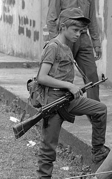
Rebel Salvadoran soldier boy combatant in Perquin, El Salvador 1990, during the Salvadoran Civil War.

During the civil war between 1980 and 1992 the Salvadoran military and the main opposition group, the Frente Farabundo Martí de Liberación National (FMLN), recruited children extensively. The recruitment was frequently carried out by force and focused on economically suppressed regions. A fifth of the army's personnel were aged under 18, as were a quarter of the FMLN. In a group of 278 former FMLN child soldiers interviewed for a study, the average age of recruitment was 10 years. The large majority of child recruits on both sides were living in poverty, and had been largely deprived of formal education. Many children who were not recruited by force joined of their own volition, mainly either to improve their circumstances or because they believed in the cause.

After the civil war came to a close, rehabilitation and reintegration programmes for children mostly failed; the majority of FMLN children were not involved in them, and the large majority of those who were dropped out of them. A decade after the peace accord former child soldiers were still experiencing nightmares, depression, anxiety, and related signs of psychiatric trauma.

Today, the Salvadoran military no longer sends children to war, but it still recruits and trains them from the age of 16.

Middle East

Iran

Detail of a propaganda mural showing a child soldier from the Iran-Iraq War, in Ardabil, Iranian Azerbaijan.

During the Iran–Iraq War (1980–1988) the armed forces used children widely; the extent of the practice is not known but the number of children involved is thought to be in the tens of thousands. Armed groups associated with the government advertised widely for male children from age 14 to join them, and the country's Supreme Leader, Ayatollah Khomeini, urged children to fight at the front. According to the Coalition to Stop the Use of Child Soldiers (now Child Soldiers International):

Ayatollah Khomeini declared that parental permission was unnecessary for those going to the front, that volunteering for military duty was a religious obligation, and that serving in the armed forces took priority over all other forms of work or study. Various sources reported that children were indoctrinated into participating in combat. They were given "keys to paradise" and promised that they would go directly to heaven if they died as martyrs against the Iraqi enemy.

The children involved were overwhelmingly from slums and poor villages, and some participated without the knowledge of their parents, including Mohammad Hossein Fahmideh. Thousands of children took part in human wave attacks, leading to widespread deaths and injuries. The total number of all Iranian casualties is estimated to be 200,000–600,000, of which approximately a third were aged 15–19 (and 3 percent under 14), according to one assessment.

After the war, the Basij, an official militia organisation, continued to recruit children from age 15, focusing on those living in poverty and sometimes recruiting them by force. In 2004, the Basij was estimated to have as many as a million members of all ages. Ansar-e Hizbollah, an armed group tolerated by the government, also recruited children widely in the 2000s, with no age restriction. As of 2018, the Iranian armed forces continue to enlist from age 16 and the government has not yet ratified the Optional Protocol on the involvement of children in armed conflict.

Iraq

The government of Saddam Hussein maintained 'boot camps' of civilian youths between the ages of 12 and 17 that involved small arms training and Ba'athist political indoctrination. Iraqi opposition sources and the US State Department reported that children who refused faced punishment. The state incorporated male children as young as ten into the Futuwah and Ashbal Saddam youth movements and then subjected them to military training, sometimes for 14 hours a day. P. W. Singer has compared the groups to the Hitler Jugend. In the Gulf War 12-year-old boys fought for the Iraqis. Children also participated in the Iran–Iraq War.

In the 2003 invasion of Iraq, US forces fought children at Nasariya, Karbala, and Kirkuk, and the US sent captured child combatants to Abu Ghraib prison. In 2009 a UN report on the post-war Iraqi occupation stated that the Iraqi insurgency had used children as combatants; it noted, for example, a suicide attack against Kirkuk's police commander by a boy aged between 10 and 13.

Asia

Cambodia

Child dressed as Khmer Rouge soldier.

In the 1970s the Khmer Rouge exploited thousands of desensitised, conscripted children in their early teens to commit mass murder and other atrocities during the Cambodian civil war and subsequent genocide. The indoctrinated children were taught to follow any order without hesitation. After it was deposed in 1979, the Khmer Rouge fought a guerrilla war against the new government, and until at least 1998 relied heavily on child recruits, including forced recruitment by abduction. During this period, the children were deployed mainly in unpaid support roles, such as ammunition-carriers, and also as combatants.

Cambodia's state armed forces also recruited children widely. Throughout the 1990s the army was recruiting children from the age of 10 and using them in armed conflict, mainly as porters and spies, and also as combatants. Four percent of the army were children, according to an estimate in the Cambodia Daily. Many children had fled the Khmer Rouge without a means to feed themselves and hoped that joining the government forces would enable them to survive, although local commanders frequently denied them any pay. Children often capitalised on the lack of an effective birth registration system to lie about their age in order to enlist. Other children, some as young as 8, were forced to join.

By 2000, the Cambodian government had signed the Optional Protocol on the Involvement of Children in Armed Conflict and its armed forces resolved to recruit adults only. Meanwhile, the Khmer Rouge had collapsed with the death of its leader, Pol Pot, in 1998. By 2004, children were no longer being recruited in the country, although the demobilisation programmes were inadequate, according to UNICEF, failing to offer appropriate rehabilitative support to released children.

Sri Lanka

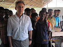
Former child soldiers at a centre for rehabilitation and reintegration into their communities, Sri Lanka.

Between 1983 and 2009 Sri Lanka's government fought a civil war with the Liberation Tigers of Tamil Eelam (Tamil Tigers). For its entire duration the Tamil Tigers and other armed groups made routine use of child recruits, typically aged 14–17 and sometimes under 10. Some children enlisted to escape deprivation or racism, or during compulsory military training at their school when they were exposed to recruitment propaganda. Others were recruited by force when walking home from school or after the Tigers pressurised families to surrender one child, as per its policy. In 2001, international sources estimated that 40 percent of Tamil Tiger personnel were children, contrary to official statements insisting that the organisation did not use them. Sri Lankan soldiers nicknamed one unit the "Baby Battalion", due to the number of children in it. Although state armed forces recruited only adults over the age of 18, they supported the Karuna group, a Tamil splinter organisation opposed to the Tamil Tigers, to recruit children by force. The government also used detained Tamil Tiger children for propaganda by exposing them to the media.

The first international initiative to demobilise and reintegrate children into their communities began in 2003, but was halted in 2004 because the Tigers failed to keep their commitment to release children from their ranks. The organisation began to release children in 2004, but continued to enlist several thousand, albeit in progressively smaller numbers, until at least 2007. The Tamil Tigers were defeated in 2009 and all other parties to the conflict stopped recruiting children in the same year.

Europe

Chechnya/Russia

During the First Chechen War, Chechen separatist forces included a large number of boys and girls, some as young as 11. According to the UN: "Child soldiers in Chechnya were reportedly assigned the same tasks as adult combatants, and served on the front lines soon after joining the armed forces." In 2004 under-18s were still believed to be involved in a range of armed groups in the war against Russia; some allegedly took part in suicide bombings.

United Kingdom

In the 20th century, the Royal Navy commonly recruited boy seamen aged from 15 up for active service; boys aged 13 or 14 were recruited for other duties.

Children aged 17 were sent to the Falklands War in 1982 (where three were killed) and the Gulf War in 1990–91 (where two were killed). 17-year-olds were also deployed as NATO peacekeepers in the former Yugoslavia during the 1990s. Having initially resisted international negotiations to prevent the deployment of children, the UK agreed to deploy adults only when it signed the Optional Protocol on the Involvement of Children in Armed Conflict in 2000, but remained committed to recruiting and training children from age 16. Between 2003 and 2010, 22 personnel aged 17 were sent to Afghanistan and Iraq, reportedly in error.

During the Troubles in Northern Ireland (c. 1960s to 1998) it was common for paramilitary groups to recruit and use children, including as combatants. Five children in Republican paramilitary groups, seven in Loyalist paramilitary groups, and five in the British armed forces, died during the conflict. The youngest, Cathleen McCartland, was recruited by the Irish Republican Army (IRA) and was aged 12 when she was killed in Belfast.

Spatial analysis

From Wikipedia, the free encyclopedia

https://en.wikipedia.org/wiki/Spatial_analysis

Map by Dr. John Snow of London, showing clusters of cholera cases in the 1854 Broad Street cholera outbreak. This was one of the first uses of map-based spatial analysis.

Spatial analysis or spatial statistics includes any of the formal techniques which studies entities using their topological, geometric, or geographic properties. Spatial analysis includes a variety of techniques, many still in their early development, using different analytic approaches and applied in fields as diverse as astronomy, with its studies of the placement of galaxies in the cosmos, to chip fabrication engineering, with its use of "place and route" algorithms to build complex wiring structures. In a more restricted sense, spatial analysis is the technique applied to structures at the human scale, most notably in the analysis of geographic data or transcriptomics data.

Complex issues arise in spatial analysis, many of which are neither clearly defined nor completely resolved, but form the basis for current research. The most fundamental of these is the problem of defining the spatial location of the entities being studied.

Classification of the techniques of spatial analysis is difficult because of the large number of different fields of research involved, the different fundamental approaches which can be chosen, and the many forms the data can take.

History

Spatial analysis began with early attempts at cartography and surveying. Land surveying goes back to at least 1,400 B.C in Egypt: the dimensions of taxable land plots were measured with measuring ropes and plumb bobs.^[1] b. Many fields have contributed to its rise in modern form. Biology contributed through botanical studies of global plant distributions and local plant locations, ethological studies of animal movement, landscape ecological studies of vegetation blocks, ecological studies of spatial population dynamics, and the study of biogeography. Epidemiology contributed with early work on disease mapping, notably John Snow's work of mapping an outbreak of cholera, with research on mapping the spread of disease and with location studies for health care delivery. Statistics has contributed greatly through work in spatial statistics. Economics has contributed notably through spatial econometrics. Geographic information system is currently a major contributor due to the importance of geographic software in the modern analytic toolbox. Remote sensing has contributed extensively in morphometric and clustering analysis. Computer science has contributed extensively through the study of algorithms, notably in computational geometry. Mathematics continues to provide the fundamental tools for analysis and to reveal the complexity of the spatial realm, for example, with recent work on fractals and scale invariance. Scientific modelling provides a useful framework for new approaches.

Fundamental issues

Spatial analysis confronts many fundamental issues in the definition of its objects of study, in the construction of the analytic operations to be used, in the use of computers for analysis, in the limitations and particularities of the analyses which are known, and in the presentation of analytic results. Many of these issues are active subjects of modern research.

Common errors often arise in spatial analysis, some due to the mathematics of space, some due to the particular ways data are presented spatially, some due to the tools which are available. Census data, because it protects individual privacy by aggregating data into local units, raises a number of statistical issues. The fractal nature of coastline makes precise measurements of its length difficult if not impossible. A computer software fitting straight lines to the curve of a coastline, can easily calculate the lengths of the lines which it defines. However these straight lines may have no inherent meaning in the real world, as was shown for the coastline of Britain.

These problems represent a challenge in spatial analysis because of the power of maps as media of presentation. When results are presented as maps, the presentation combines spatial data which are generally accurate with analytic results which may be inaccurate, leading to an impression that analytic results are more accurate than the data would indicate.

Spatial characterization

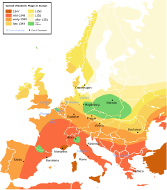
Spread of bubonic plague in medieval Europe. The colors indicate the spatial distribution of plague outbreaks over time.

The definition of the spatial presence of an entity constrains the possible analysis which can be applied to that entity and influences the final conclusions that can be reached. While this property is fundamentally true of all analysis, it is particularly important in spatial analysis because the tools to define and study entities favor specific characterizations of the entities being studied. Statistical techniques favor the spatial definition of objects as points because there are very few statistical techniques which operate directly on line, area, or volume elements. Computer tools favor the spatial definition of objects as homogeneous and separate elements because of the limited number of database elements and computational structures available, and the ease with which these primitive structures can be created.

Spatial dependence

Spatial dependence is the spatial relationship of variable values (for themes defined over space, such as rainfall) or locations (for themes defined as objects, such as cities). Spatial dependence is measured as the existence of statistical dependence in a collection of random variables, each of which is associated with a different geographical location. Spatial dependence is of importance in applications where it is reasonable to postulate the existence of corresponding set of random variables at locations that have not been included in a sample. Thus rainfall may be measured at a set of rain gauge locations, and such measurements can be considered as outcomes of random variables, but rainfall clearly occurs at other locations and would again be random. Because rainfall exhibits properties of autocorrelation, spatial interpolation techniques can be used to estimate rainfall amounts at locations near measured locations.

As with other types of statistical dependence, the presence of spatial dependence generally leads to estimates of an average value from a sample being less accurate than had the samples been independent, although if negative dependence exists a sample average can be better than in the independent case. A different problem than that of estimating an overall average is that of spatial interpolation: here the problem is to estimate the unobserved random outcomes of variables at locations intermediate to places where measurements are made, on that there is spatial dependence between the observed and unobserved random variables.

Tools for exploring spatial dependence include: spatial correlation, spatial covariance functions and semivariograms. Methods for spatial interpolation include Kriging, which is a type of best linear unbiased prediction. The topic of spatial dependence is of importance to geostatistics and spatial analysis.

Spatial auto-correlation

Spatial dependency is the co-variation of properties within geographic space: characteristics at proximal locations appear to be correlated, either positively or negatively. Spatial dependency leads to the spatial autocorrelation problem in statistics since, like temporal autocorrelation, this violates standard statistical techniques that assume independence among observations. For example, regression analyses that do not compensate for spatial dependency can have unstable parameter estimates and yield unreliable significance tests. Spatial regression models (see below) capture these relationships and do not suffer from these weaknesses. It is also appropriate to view spatial dependency as a source of information rather than something to be corrected.

Locational effects also manifest as spatial heterogeneity, or the apparent variation in a process with respect to location in geographic space. Unless a space is uniform and boundless, every location will have some degree of uniqueness relative to the other locations. This affects the spatial dependency relations and therefore the spatial process. Spatial heterogeneity means that overall parameters estimated for the entire system may not adequately describe the process at any given location.

Spatial association

Spatial association is the degree to which things are similarly arranged in space. Analysis of the distribution patterns of two phenomena is done by map overlay. If the distributions are similar, then the spatial association is strong, and vice versa. In a Geographic Information System, the analysis can be done quantitatively. For example, a set of observations (as points or extracted from raster cells) at matching locations can be intersected and examined by regression analysis.

Like spatial autocorrelation, this can be a useful tool for spatial prediction. In spatial modeling, the concept of spatial association allows the use of covariates in a regression equation to predict the geographic field and thus produce a map.

Scaling

Spatial measurement scale is a persistent issue in spatial analysis; more detail is available at the modifiable areal unit problem (MAUP) topic entry. Landscape ecologists developed a series of scale invariant metrics for aspects of ecology that are fractal in nature. In more general terms, no scale independent method of analysis is widely agreed upon for spatial statistics.

Sampling

Spatial sampling involves determining a limited number of locations in geographic space for faithfully measuring phenomena that are subject to dependency and heterogeneity. Dependency suggests that since one location can predict the value of another location, we do not need observations in both places. But heterogeneity suggests that this relation can change across space, and therefore we cannot trust an observed degree of dependency beyond a region that may be small. Basic spatial sampling schemes include random, clustered and systematic. These basic schemes can be applied at multiple levels in a designated spatial hierarchy (e.g., urban area, city, neighborhood). It is also possible to exploit ancillary data, for example, using property values as a guide in a spatial sampling scheme to measure educational attainment and income. Spatial models such as autocorrelation statistics, regression and interpolation (see below) can also dictate sample design.

Common errors in spatial analysis

The fundamental issues in spatial analysis lead to numerous problems in analysis including bias, distortion and outright errors in the conclusions reached. These issues are often interlinked but various attempts have been made to separate out particular issues from each other.

Length

In discussing the coastline of Britain, Benoit Mandelbrot showed that certain spatial concepts are inherently nonsensical despite presumption of their validity. Lengths in ecology depend directly on the scale at which they are measured and experienced. So while surveyors commonly measure the length of a river, this length only has meaning in the context of the relevance of the measuring technique to the question under study.

Britain measured using a 200km linear measurement
Britain measured using a 100km linear measurement
Britain measured using a 50km linear measurement

Locational fallacy

The locational fallacy refers to error due to the particular spatial characterization chosen for the elements of study, in particular choice of placement for the spatial presence of the element.

Spatial characterizations may be simplistic or even wrong. Studies of humans often reduce the spatial existence of humans to a single point, for instance their home address. This can easily lead to poor analysis, for example, when considering disease transmission which can happen at work or at school and therefore far from the home.

The spatial characterization may implicitly limit the subject of study. For example, the spatial analysis of crime data has recently become popular but these studies can only describe the particular kinds of crime which can be described spatially. This leads to many maps of assault but not to any maps of embezzlement with political consequences in the conceptualization of crime and the design of policies to address the issue.

Atomic fallacy

This describes errors due to treating elements as separate 'atoms' outside of their spatial context. The fallacy is about transferring individual conclusions to spatial units.

Ecological fallacy

The ecological fallacy describes errors due to performing analyses on aggregate data when trying to reach conclusions on the individual units. Errors occur in part from spatial aggregation. For example, a pixel represents the average surface temperatures within an area. Ecological fallacy would be to assume that all points within the area have the same temperature.

Solutions to the fundamental issues

Geographic space

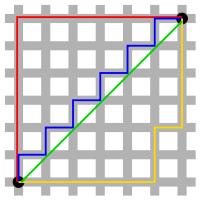
Manhattan distance versus Euclidean distance: The red, blue, and yellow lines have the same length (12) in both Euclidean and taxicab geometry. In Euclidean geometry, the green line has length 6×√2 ≈ 8.48, and is the unique shortest path. In taxicab geometry, the green line's length is still 12, making it no shorter than any other path shown.

A mathematical space exists whenever we have a set of observations and quantitative measures of their attributes. For example, we can represent individuals' incomes or years of education within a coordinate system where the location of each individual can be specified with respect to both dimensions. The distance between individuals within this space is a quantitative measure of their differences with respect to income and education. However, in spatial analysis, we are concerned with specific types of mathematical spaces, namely, geographic space. In geographic space, the observations correspond to locations in a spatial measurement framework that capture their proximity in the real world. The locations in a spatial measurement framework often represent locations on the surface of the Earth, but this is not strictly necessary. A spatial measurement framework can also capture proximity with respect to, say, interstellar space or within a biological entity such as a liver. The fundamental tenet is Tobler's First Law of Geography: if the interrelation between entities increases with proximity in the real world, then representation in geographic space and assessment using spatial analysis techniques are appropriate.

The Euclidean distance between locations often represents their proximity, although this is only one possibility. There are an infinite number of distances in addition to Euclidean that can support quantitative analysis. For example, "Manhattan" (or "Taxicab") distances where movement is restricted to paths parallel to the axes can be more meaningful than Euclidean distances in urban settings. In addition to distances, other geographic relationships such as connectivity (e.g., the existence or degree of shared borders) and direction can also influence the relationships among entities. It is also possible to compute minimal cost paths across a cost surface; for example, this can represent proximity among locations when travel must occur across rugged terrain.

Types

Spatial data comes in many varieties and it is not easy to arrive at a system of classification that is simultaneously exclusive, exhaustive, imaginative, and satisfying. -- G. Upton & B. Fingelton

Spatial data analysis

Urban and Regional Studies deal with large tables of spatial data obtained from censuses and surveys. It is necessary to simplify the huge amount of detailed information in order to extract the main trends. Multivariable analysis (or Factor analysis, FA) allows a change of variables, transforming the many variables of the census, usually correlated between themselves, into fewer independent "Factors" or "Principal Components" which are, actually, the eigenvectors of the data correlation matrix weighted by the inverse of their eigenvalues. This change of variables has two main advantages:

Since information is concentrated on the first new factors, it is possible to keep only a few of them while losing only a small amount of information; mapping them produces fewer and more significant maps
The factors, actually the eigenvectors, are orthogonal by construction, i.e. not correlated. In most cases, the dominant factor (with the largest eigenvalue) is the Social Component, separating rich and poor in the city. Since factors are not-correlated, other smaller processes than social status, which would have remained hidden otherwise, appear on the second, third, ... factors.

Factor analysis depends on measuring distances between observations : the choice of a significant metric is crucial. The Euclidean metric (Principal Component Analysis), the Chi-Square distance (Correspondence Analysis) or the Generalized Mahalanobis distance (Discriminant Analysis) are among the more widely used. More complicated models, using communalities or rotations have been proposed.

Using multivariate methods in spatial analysis began really in the 1950s (although some examples go back to the beginning of the century) and culminated in the 1970s, with the increasing power and accessibility of computers. Already in 1948, in a seminal publication, two sociologists, Wendell Bell and Eshref Shevky, had shown that most city populations in the US and in the world could be represented with three independent factors : 1- the « socio-economic status » opposing rich and poor districts and distributed in sectors running along highways from the city center, 2- the « life cycle », i.e. the age structure of households, distributed in concentric circles, and 3- « race and ethnicity », identifying patches of migrants located within the city. In 1961, in a groundbreaking study, British geographers used FA to classify British towns. Brian J Berry, at the University of Chicago, and his students made a wide use of the method, applying it to most important cities in the world and exhibiting common social structures. The use of Factor Analysis in Geography, made so easy by modern computers, has been very wide but not always very wise.

Since the vectors extracted are determined by the data matrix, it is not possible to compare factors obtained from different censuses. A solution consists in fusing together several census matrices in a unique table which, then, may be analyzed. This, however, assumes that the definition of the variables has not changed over time and produces very large tables, difficult to manage. A better solution, proposed by psychometricians, groups the data in a « cubic matrix », with three entries (for instance, locations, variables, time periods). A Three-Way Factor Analysis produces then three groups of factors related by a small cubic « core matrix ». This method, which exhibits data evolution over time, has not been widely used in geography. In Los Angeles, however, it has exhibited the role, traditionally ignored, of Downtown as an organizing center for the whole city during several decades.

Spatial autocorrelation

Spatial autocorrelation statistics measure and analyze the degree of dependency among observations in a geographic space. Classic spatial autocorrelation statistics include Moran's $I$ , Geary's $C$ , Getis's $G$ and the standard deviational ellipse. These statistics require measuring a spatial weights matrix that reflects the intensity of the geographic relationship between observations in a neighborhood, e.g., the distances between neighbors, the lengths of shared border, or whether they fall into a specified directional class such as "west". Classic spatial autocorrelation statistics compare the spatial weights to the covariance relationship at pairs of locations. Spatial autocorrelation that is more positive than expected from random indicate the clustering of similar values across geographic space, while significant negative spatial autocorrelation indicates that neighboring values are more dissimilar than expected by chance, suggesting a spatial pattern similar to a chess board.

Spatial autocorrelation statistics such as Moran's $I$ and Geary's $C$ are global in the sense that they estimate the overall degree of spatial autocorrelation for a dataset. The possibility of spatial heterogeneity suggests that the estimated degree of autocorrelation may vary significantly across geographic space. Local spatial autocorrelation statistics provide estimates disaggregated to the level of the spatial analysis units, allowing assessment of the dependency relationships across space. $G$ statistics compare neighborhoods to a global average and identify local regions of strong autocorrelation. Local versions of the $I$ and $C$ statistics are also available.

Spatial heterogeneity

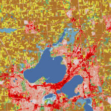
Land cover surrounding Madison, WI. Fields are colored yellow and brown, water is colored blue, and urban surfaces are colored red.

Spatial heterogeneity is a property generally ascribed to a landscape or to a population. It refers to the uneven distribution of various concentrations of each species within an area. A landscape with spatial heterogeneity has a mix of concentrations of multiple species of plants or animals (biological), or of terrain formations (geological), or environmental characteristics (e.g. rainfall, temperature, wind) filling its area. A population showing spatial heterogeneity is one where various concentrations of individuals of this species are unevenly distributed across an area; nearly synonymous with "patchily distributed."

Spatial interpolation

Spatial interpolation methods estimate the variables at unobserved locations in geographic space based on the values at observed locations. Basic methods include inverse distance weighting: this attenuates the variable with decreasing proximity from the observed location. Kriging is a more sophisticated method that interpolates across space according to a spatial lag relationship that has both systematic and random components. This can accommodate a wide range of spatial relationships for the hidden values between observed locations. Kriging provides optimal estimates given the hypothesized lag relationship, and error estimates can be mapped to determine if spatial patterns exist.

Spatial regression

Spatial regression methods capture spatial dependency in regression analysis, avoiding statistical problems such as unstable parameters and unreliable significance tests, as well as providing information on spatial relationships among the variables involved. Depending on the specific technique, spatial dependency can enter the regression model as relationships between the independent variables and the dependent, between the dependent variables and a spatial lag of itself, or in the error terms. Geographically weighted regression (GWR) is a local version of spatial regression that generates parameters disaggregated by the spatial units of analysis. This allows assessment of the spatial heterogeneity in the estimated relationships between the independent and dependent variables. The use of Bayesian hierarchical modeling in conjunction with Markov chain Monte Carlo (MCMC) methods have recently shown to be effective in modeling complex relationships using Poisson-Gamma-CAR, Poisson-lognormal-SAR, or Overdispersed logit models. Statistical packages for implementing such Bayesian models using MCMC include WinBugs, CrimeStat and many packages available via R programming language.

Spatial stochastic processes, such as Gaussian processes are also increasingly being deployed in spatial regression analysis. Model-based versions of GWR, known as spatially varying coefficient models have been applied to conduct Bayesian inference. Spatial stochastic process can become computationally effective and scalable Gaussian process models, such as Gaussian Predictive Processes and Nearest Neighbor Gaussian Processes (NNGP).

Spatial interaction

Spatial interaction or "gravity models" estimate the flow of people, material or information between locations in geographic space. Factors can include origin propulsive variables such as the number of commuters in residential areas, destination attractiveness variables such as the amount of office space in employment areas, and proximity relationships between the locations measured in terms such as driving distance or travel time. In addition, the topological, or connective, relationships between areas must be identified, particularly considering the often conflicting relationship between distance and topology; for example, two spatially close neighborhoods may not display any significant interaction if they are separated by a highway. After specifying the functional forms of these relationships, the analyst can estimate model parameters using observed flow data and standard estimation techniques such as ordinary least squares or maximum likelihood. Competing destinations versions of spatial interaction models include the proximity among the destinations (or origins) in addition to the origin-destination proximity; this captures the effects of destination (origin) clustering on flows. Computational methods such as artificial neural networks can also estimate spatial interaction relationships among locations and can handle noisy and qualitative data.

Simulation and modeling

Spatial interaction models are aggregate and top-down: they specify an overall governing relationship for flow between locations. This characteristic is also shared by urban models such as those based on mathematical programming, flows among economic sectors, or bid-rent theory. An alternative modeling perspective is to represent the system at the highest possible level of disaggregation and study the bottom-up emergence of complex patterns and relationships from behavior and interactions at the individual level.

Complex adaptive systems theory as applied to spatial analysis suggests that simple interactions among proximal entities can lead to intricate, persistent and functional spatial entities at aggregate levels. Two fundamentally spatial simulation methods are cellular automata and agent-based modeling. Cellular automata modeling imposes a fixed spatial framework such as grid cells and specifies rules that dictate the state of a cell based on the states of its neighboring cells. As time progresses, spatial patterns emerge as cells change states based on their neighbors; this alters the conditions for future time periods. For example, cells can represent locations in an urban area and their states can be different types of land use. Patterns that can emerge from the simple interactions of local land uses include office districts and urban sprawl. Agent-based modeling uses software entities (agents) that have purposeful behavior (goals) and can react, interact and modify their environment while seeking their objectives. Unlike the cells in cellular automata, simulysts can allow agents to be mobile with respect to space. For example, one could model traffic flow and dynamics using agents representing individual vehicles that try to minimize travel time between specified origins and destinations. While pursuing minimal travel times, the agents must avoid collisions with other vehicles also seeking to minimize their travel times. Cellular automata and agent-based modeling are complementary modeling strategies. They can be integrated into a common geographic automata system where some agents are fixed while others are mobile.

Calibration plays a pivotal role in both CA and ABM simulation and modelling approaches. Initial approaches to CA proposed robust calibration approaches based on stochastic, Monte Carlo methods. ABM approaches rely on agents' decision rules (in many cases extracted from qualitative research base methods such as questionnaires). Recent Machine Learning Algorithms calibrate using training sets, for instance in order to understand the qualities of the built environment.

Multiple-point geostatistics (MPS)

Spatial analysis of a conceptual geological model is the main purpose of any MPS algorithm. The method analyzes the spatial statistics of the geological model, called the training image, and generates realizations of the phenomena that honor those input multiple-point statistics.

A recent MPS algorithm used to accomplish this task is the pattern-based method by Honarkhah. In this method, a distance-based approach is employed to analyze the patterns in the training image. This allows the reproduction of the multiple-point statistics, and the complex geometrical features of the training image. Each output of the MPS algorithm is a realization that represents a random field. Together, several realizations may be used to quantify spatial uncertainty.

One of the recent methods is presented by Tahmasebi et al. uses a cross-correlation function to improve the spatial pattern reproduction. They call their MPS simulation method as the CCSIM algorithm. This method is able to quantify the spatial connectivity, variability and uncertainty. Furthermore, the method is not sensitive to any type of data and is able to simulate both categorical and continuous scenarios. CCSIM algorithm is able to be used for any stationary, non-stationary and multivariate systems and it can provide high quality visual appeal model.

Geospatial and hydrospatial analysis

Geospatial and hydrospatial analysis, or just spatial analysis, is an approach to applying statistical analysis and other analytic techniques to data which has a geographical or spatial aspect. Such analysis would typically employ software capable of rendering maps processing spatial data, and applying analytical methods to terrestrial or geographic datasets, including the use of geographic information systems and geomatics.

Geographical information system usage

Geographic information systems (GIS) — a large domain that provides a variety of capabilities designed to capture, store, manipulate, analyze, manage, and present all types of geographical data — utilizes geospatial and hydrospatial analysis in a variety of contexts, operations and applications.

Basic applications

Geospatial and Hydrospatial analysis, using GIS, was developed for problems in the environmental and life sciences, in particular ecology, geology and epidemiology. It has extended to almost all industries including defense, intelligence, utilities, Natural Resources (i.e. Oil and Gas, Forestry ... etc.), social sciences, medicine and Public Safety (i.e. emergency management and criminology), disaster risk reduction and management (DRRM), and climate change adaptation (CCA). Spatial statistics typically result primarily from observation rather than experimentation. Hydrospatial is particularly used for the aquatic side and the members related to the water surface, column, bottom, sub-bottom and the coastal zones.

Basic operations

Vector-based GIS is typically related to operations such as map overlay (combining two or more maps or map layers according to predefined rules), simple buffering (identifying regions of a map within a specified distance of one or more features, such as towns, roads or rivers) and similar basic operations. This reflects (and is reflected in) the use of the term spatial analysis within the Open Geospatial Consortium (OGC) “simple feature specifications”. For raster-based GIS, widely used in the environmental sciences and remote sensing, this typically means a range of actions applied to the grid cells of one or more maps (or images) often involving filtering and/or algebraic operations (map algebra). These techniques involve processing one or more raster layers according to simple rules resulting in a new map layer, for example replacing each cell value with some combination of its neighbours’ values, or computing the sum or difference of specific attribute values for each grid cell in two matching raster datasets. Descriptive statistics, such as cell counts, means, variances, maxima, minima, cumulative values, frequencies and a number of other measures and distance computations are also often included in this generic term spatial analysis. Spatial analysis includes a large variety of statistical techniques (descriptive, exploratory, and explanatory statistics) that apply to data that vary spatially and which can vary over time. Some more advanced statistical techniques include Getis-ord Gi* or Anselin Local Moran's I which are used to determine clustering patterns of spatially referenced data.

Advanced operations

Geospatial and Hydrospatial analysis goes beyond 2D and 3D mapping operations and spatial statistics. It is multi-dimensional and also temporal and includes:

Surface analysis — in particular analysing the properties of physical surfaces, such as gradient, aspect and visibility, and analysing surface-like data “fields”;
Network analysis — examining the properties of natural and man-made networks in order to understand the behaviour of flows within and around such networks; and locational analysis. GIS-based network analysis may be used to address a wide range of practical problems such as route selection and facility location (core topics in the field of operations research), and problems involving flows such as those found in Hydrospatial and hydrology and transportation research. In many instances location problems relate to networks and as such are addressed with tools designed for this purpose, but in others existing networks may have little or no relevance or may be impractical to incorporate within the modeling process. Problems that are not specifically network constrained, such as new road or pipeline routing, regional warehouse location, mobile phone mast positioning or the selection of rural community health care sites, may be effectively analysed (at least initially) without reference to existing physical networks. Locational analysis "in the plane" is also applicable where suitable network datasets are not available, or are too large or expensive to be utilised, or where the location algorithm is very complex or involves the examination or simulation of a very large number of alternative configurations.
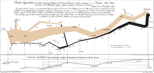
Geovisualization — the creation and manipulation of images, maps, diagrams, charts, 3D views and their associated tabular datasets. GIS packages increasingly provide a range of such tools, providing static or rotating views, draping images over 2.5D surface representations, providing animations and fly-throughs, dynamic linking and brushing and spatio-temporal visualisations. This latter class of tools is the least developed, reflecting in part the limited range of suitable compatible datasets and the limited set of analytical methods available, although this picture is changing rapidly. All these facilities augment the core tools utilised in spatial analysis throughout the analytical process (exploration of data, identification of patterns and relationships, construction of models, and communication of results)

Mobile geospatial and hydrospatial Computing

Traditionally geospatial and hydrospatial computing has been performed primarily on personal computers (PCs) or servers. Due to the increasing capabilities of mobile devices, however, geospatial computing in mobile devices is a fast-growing trend. The portable nature of these devices, as well as the presence of useful sensors, such as Global Navigation Satellite System (GNSS) receivers and barometric pressure sensors, make them useful for capturing and processing geospatial and hydrospatial information in the field. In addition to the local processing of geospatial information on mobile devices, another growing trend is cloud-based geospatial computing. In this architecture, data can be collected in the field using mobile devices and then transmitted to cloud-based servers for further processing and ultimate storage. In a similar manner, geospatial and hydrospatial information can be made available to connected mobile devices via the cloud, allowing access to vast databases of geospatial and hydrospatial information anywhere where a wireless data connection is available.

Geographic information science and spatial analysis

This flow map of Napoleon's ill-fated march on Moscow is an early and celebrated example of geovisualization. It shows the army's direction as it traveled, the places the troops passed through, the size of the army as troops died from hunger and wounds, and the freezing temperatures they experienced.

Geographic information systems (GIS) and the underlying geographic information science that advances these technologies have a strong influence on spatial analysis. The increasing ability to capture and handle geographic data means that spatial analysis is occurring within increasingly data-rich environments. Geographic data capture systems include remotely sensed imagery, environmental monitoring systems such as intelligent transportation systems, and location-aware technologies such as mobile devices that can report location in near-real time. GIS provide platforms for managing these data, computing spatial relationships such as distance, connectivity and directional relationships between spatial units, and visualizing both the raw data and spatial analytic results within a cartographic context. Subtypes include:

Geovisualization (GVis) combines scientific visualization with digital cartography to support the exploration and analysis of geographic data and information, including the results of spatial analysis or simulation. GVis leverages the human orientation towards visual information processing in the exploration, analysis and communication of geographic data and information. In contrast with traditional cartography, GVis is typically three- or four-dimensional (the latter including time) and user-interactive.
Geographic knowledge discovery (GKD) is the human-centered process of applying efficient computational tools for exploring massive spatial databases. GKD includes geographic data mining, but also encompasses related activities such as data selection, data cleaning and pre-processing, and interpretation of results. GVis can also serve a central role in the GKD process. GKD is based on the premise that massive databases contain interesting (valid, novel, useful and understandable) patterns that standard analytical techniques cannot find. GKD can serve as a hypothesis-generating process for spatial analysis, producing tentative patterns and relationships that should be confirmed using spatial analytical techniques.
Spatial decision support systems (SDSS) take existing spatial data and use a variety of mathematical models to make projections into the future. This allows urban and regional planners to test intervention decisions prior to implementation.

Search This Blog