A Medley of Potpourri

Tuesday, September 21, 2021

Climate change feedback

From Wikipedia, the free encyclopedia

https://en.wikipedia.org/wiki/Climate_change_feedback

The primary causes and the wide-ranging effects of global warming and resulting climate change. Some effects constitute feedback mechanisms that intensify climate change and move it toward climate tipping points.

Climate change feedbacks are important in the understanding of global warming because feedback processes amplify or diminish the effect of each climate forcing, and so play an important part in determining the climate sensitivity and future climate state. Feedback in general is the process in which changing one quantity changes a second quantity, and the change in the second quantity in turn changes the first. Positive (or reinforcing) feedback amplifies the change in the first quantity while negative (or balancing) feedback reduces it.

The term "forcing" means a change which may "push" the climate system in the direction of warming or cooling. An example of a climate forcing is increased atmospheric concentrations of greenhouse gases. By definition, forcings are external to the climate system while feedbacks are internal; in essence, feedbacks represent the internal processes of the system. Some feedbacks may act in relative isolation to the rest of the climate system; others may be tightly coupled; hence it may be difficult to tell just how much a particular process contributes. Forcing can also be driven by socioeconomic factors such as "demand for biofuels or demand for soy bean production." These drivers work as forcing mechanisms by the direct and indirect effects they cause from an individual to a global scale.

Forcings and feedbacks together determine how much and how fast the climate changes. The main positive feedback in global warming is the tendency of warming to increase the amount of water vapor in the atmosphere, which in turn leads to further warming. The main negative feedback comes from the Stefan–Boltzmann law, the amount of heat radiated from the Earth into space changes with the fourth power of the temperature of Earth's surface and atmosphere. Observations and modelling studies indicate that there is a net positive feedback to warming. Large positive feedbacks can lead to effects that are abrupt or irreversible, depending upon the rate and magnitude of the climate change.

Positive

Carbon cycle feedbacks

There have been predictions, and some evidence, that global warming might cause loss of carbon from terrestrial ecosystems, leading to an increase of atmospheric CO
2 levels. Several climate models indicate that global warming through the 21st century could be accelerated by the response of the terrestrial carbon cycle to such warming. All 11 models in the C4MIP study found that a larger fraction of anthropogenic CO₂ will stay airborne if climate change is accounted for. By the end of the twenty-first century, this additional CO₂ varied between 20 and 200 ppm for the two extreme models, the majority of the models lying between 50 and 100 ppm. The higher CO₂ levels led to an additional climate warming ranging between 0.1° and 1.5 °C. However, there was still a large uncertainty on the magnitude of these sensitivities. Eight models attributed most of the changes to the land, while three attributed it to the ocean. The strongest feedbacks in these cases are due to increased respiration of carbon from soils throughout the high latitude boreal forests of the Northern Hemisphere. One model in particular (HadCM3) indicates a secondary carbon cycle feedback due to the loss of much of the Amazon Rainforest in response to significantly reduced precipitation over tropical South America. While models disagree on the strength of any terrestrial carbon cycle feedback, they each suggest any such feedback would accelerate global warming.

Observations show that soils in the U.K have been losing carbon at the rate of four million tonnes a year for the past 25 years according to a paper in Nature by Bellamy et al. in September 2005, who note that these results are unlikely to be explained by land use changes. Results such as this rely on a dense sampling network and thus are not available on a global scale. Extrapolating to all of the United Kingdom, they estimate annual losses of 13 million tons per year. This is as much as the annual reductions in carbon dioxide emissions achieved by the UK under the Kyoto Treaty (12.7 million tons of carbon per year).

It has also been suggested (by Chris Freeman) that the release of dissolved organic carbon (DOC) from peat bogs into water courses (from which it would in turn enter the atmosphere) constitutes a positive feedback for global warming. The carbon currently stored in peatlands (390–455 gigatonnes, one-third of the total land-based carbon store) is over half the amount of carbon already in the atmosphere. DOC levels in water courses are observably rising; Freeman's hypothesis is that, not elevated temperatures, but elevated levels of atmospheric CO₂ are responsible, through stimulation of primary productivity.

Tree deaths are believed to be increasing as a result of climate change, which is a positive feedback effect.

Methane climate feedbacks in natural ecosystems.

Wetlands and freshwater ecosystems are predicted to be the largest potential contributor to a global methane climate feedback. Long-term warming changes the balance in the methane-related microbial community within freshwater ecosystems so they produce more methane while proportionately less is oxidised to carbon dioxide.

Arctic methane release

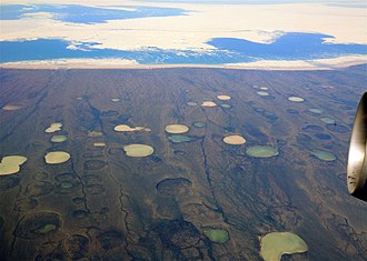
Photo shows what appears to be permafrost thaw ponds in Hudson Bay, Canada, near Greenland. (2008) Global warming will increase permafrost and peatland thaw, which can result in collapse of plateau surfaces.

Warming is also the triggering variable for the release of carbon (potentially as methane) in the arctic. Methane released from thawing permafrost such as the frozen peat bogs in Siberia, and from methane clathrate on the sea floor, creates a positive feedback. In April 2019, Turetsky et al. reported permafrost was thawing quicker than predicted. Recently the understanding of the climate feedback from permafrost improved, but potential emissions from the subsea permafrost remain unknown and are - like many other soil carbon feedbacks - still absent from most climate models.

Thawing permafrost peat bogs

Western Siberia is the world's largest peat bog, a one million square kilometer region of permafrost peat bog that was formed 11,000 years ago at the end of the last ice age. The melting of its permafrost is likely to lead to the release, over decades, of large quantities of methane. As much as 70,000 million tonnes of methane, an extremely effective greenhouse gas, might be released over the next few decades, creating an additional source of greenhouse gas emissions. Similar melting has been observed in eastern Siberia. Lawrence et al. (2008) suggest that a rapid melting of Arctic sea ice may start a feedback loop that rapidly melts Arctic permafrost, triggering further warming. May 31, 2010. NASA published that globally "Greenhouse gases are escaping the permafrost and entering the atmosphere at an increasing rate - up to 50 billion tons each year of methane, for example - due to a global thawing trend. This is particularly troublesome because methane heats the atmosphere with 25 times the efficiency of carbon dioxide" (the equivalent of 1250 billion tons of CO
2 per year).

In 2019, a report called " Arctic report card " estimated the current greenhouse gas emissions from Arctic permafrost as almost equal to the emissions of Russia or Japan or less than 10% of the global emissions from fossil fuels.

Hydrates

Methane clathrate, also called methane hydrate, is a form of water ice that contains a large amount of methane within its crystal structure. Extremely large deposits of methane clathrate have been found under sediments on the sea and ocean floors of Earth. The sudden release of large amounts of natural gas from methane clathrate deposits, in a runaway global warming event, has been hypothesized as a cause of past and possibly future climate changes. The release of this trapped methane is a potential major outcome of a rise in temperature; it is thought that this might increase the global temperature by an additional 5° in itself, as methane is much more powerful as a greenhouse gas than carbon dioxide. The theory also predicts this will greatly affect available oxygen content of the atmosphere. This theory has been proposed to explain the most severe mass extinction event on earth known as the Permian–Triassic extinction event, and also the Paleocene-Eocene Thermal Maximum climate change event. In 2008, a research expedition for the American Geophysical Union detected levels of methane up to 100 times above normal in the Siberian Arctic, likely being released by methane clathrates being released by holes in a frozen 'lid' of seabed permafrost, around the outfall of the Lena River and the area between the Laptev Sea and East Siberian Sea.

In 2020, the first leak of methane from the sea floor in Antarctica was discovered. The scientists are not sure what caused it. The area where it was found had not warmed yet significantly. It is on the side of a volcano, but it seems that it is not from there. The methane - eating microbes, eat the methane much fewer that was supposed, and the researchers think this should be included in climate models. They also claim that there is much more to discover about the issue in Antarctica. A quarter of all marine methane is found in the region of Antarctica

Abrupt increases in atmospheric methane

Literature assessments by the Intergovernmental Panel on Climate Change (IPCC) and the US Climate Change Science Program (CCSP) have considered the possibility of future projected climate change leading to a rapid increase in atmospheric methane. The IPCC Third Assessment Report, published in 2001, looked at possible rapid increases in methane due either to reductions in the atmospheric chemical sink or from the release of buried methane reservoirs. In both cases, it was judged that such a release would be "exceptionally unlikely" (less than a 1% chance, based on expert judgement). The CCSP assessment, published in 2008, concluded that an abrupt release of methane into the atmosphere appeared "very unlikely" (less than 10% probability, based on expert judgement). The CCSP assessment, however, noted that climate change would "very likely" (greater than 90% probability, based on expert judgement) accelerate the pace of persistent emissions from both hydrate sources and wetlands.

On 10 June 2019 Louise M. Farquharson and her team reported that their 12-year study into Canadian permafrost had "Observed maximum thaw depths at our sites are already exceeding those projected to occur by 2090. Between 1990 and 2016, an increase of up to 4 °C has been observed in terrestrial permafrost and this trend is expected to continue as Arctic mean annual air temperatures increase at a rate twice that of lower latitudes." Determining the extent of new thermokarst development is difficult, but there is little doubt the problem is widespread. Farquharson and her team guess that about 231,000 square miles (600,000 square kilometers) of permafrost, or about 5.5% of the zone that is permafrost year-round, is vulnerable to rapid surface thawing.

Decomposition

Organic matter stored in permafrost generates heat as it decomposes in response to the permafrost melting. As the tropics get wetter, as many climate models predict, soils are likely to experience greater rates of respiration and decomposition, limiting the carbon storage abilities of tropical soils.

Peat decomposition

Peat, occurring naturally in peat bogs, is a store of carbon significant on a global scale. When peat dries it decomposes, and may additionally burn. Water table adjustment due to global warming may cause significant excursions of carbon from peat bogs. This may be released as methane, which can exacerbate the feedback effect, due to its high global warming potential.

Rainforest drying

Rainforests, most notably tropical rainforests, are particularly vulnerable to global warming. There are a number of effects which may occur, but two are particularly concerning. Firstly, the drier vegetation may cause total collapse of the rainforest ecosystem. For example, the Amazon rainforest would tend to be replaced by caatinga ecosystems. Further, even tropical rainforests ecosystems which do not collapse entirely may lose significant proportions of their stored carbon as a result of drying, due to changes in vegetation.

Forest fires

The IPCC Fourth Assessment Report predicts that many mid-latitude regions, such as Mediterranean Europe, will experience decreased rainfall and an increased risk of drought, which in turn would allow forest fires to occur on larger scale, and more regularly. This releases more stored carbon into the atmosphere than the carbon cycle can naturally re-absorb, as well as reducing the overall forest area on the planet, creating a positive feedback loop. Part of that feedback loop is more rapid growth of replacement forests and a northward migration of forests as northern latitudes become more suitable climates for sustaining forests. There is a question of whether the burning of renewable fuels such as forests should be counted as contributing to global warming. Cook & Vizy also found that forest fires were likely in the Amazon Rainforest, eventually resulting in a transition to Caatinga vegetation in the Eastern Amazon region.

Desertification

Desertification is a consequence of global warming in some environments. Desert soils contain little humus, and support little vegetation. As a result, transition to desert ecosystems is typically associated with excursions of carbon.

Modelling results

The global warming projections contained in the IPCC's Fourth Assessment Report (AR4) include carbon cycle feedbacks. Authors of AR4, however, noted that scientific understanding of carbon cycle feedbacks was poor. Projections in AR4 were based on a range of greenhouse gas emissions scenarios, and suggested warming between the late 20th and late 21st century of 1.1 to 6.4 °C. This is the "likely" range (greater than 66% probability), based on the expert judgement of the IPCC's authors. Authors noted that the lower end of the "likely" range appeared to be better constrained than the upper end of the "likely" range, in part due to carbon cycle feedbacks. The American Meteorological Society has commented that more research is needed to model the effects of carbon cycle feedbacks in climate change projections.

Isaken et al. (2010) considered how future methane release from the Arctic might contribute to global warming. Their study suggested that if global methane emissions were to increase by a factor of 2.5 to 5.2 above (then) current emissions, the indirect contribution to radiative forcing would be about 250% and 400% respectively, of the forcing that can be directly attributed to methane. This amplification of methane warming is due to projected changes in atmospheric chemistry.

Schaefer et al. (2011) considered how carbon released from permafrost might contribute to global warming. Their study projected changes in permafrost based on a medium greenhouse gas emissions scenario (SRES A1B). According to the study, by 2200, the permafrost feedback might contribute 190 (+/- 64) gigatons of carbon cumulatively to the atmosphere. Schaefer et al. (2011) commented that this estimate may be low.

Implications for climate policy

Uncertainty over climate change feedbacks has implications for climate policy. For instance, uncertainty over carbon cycle feedbacks may affect targets for reducing greenhouse gas emissions. Emissions targets are often based on a target stabilization level of atmospheric greenhouse gas concentrations, or on a target for limiting global warming to a particular magnitude. Both of these targets (concentrations or temperatures) require an understanding of future changes in the carbon cycle. If models incorrectly project future changes in the carbon cycle, then concentration or temperature targets could be missed. For example, if models underestimate the amount of carbon released into the atmosphere due to positive feedbacks (e.g., due to melting permafrost), then they may also underestimate the extent of emissions reductions necessary to meet a concentration or temperature target.

Cloud feedback

Warming is expected to change the distribution and type of clouds. Seen from below, clouds emit infrared radiation back to the surface, and so exert a warming effect; seen from above, clouds reflect sunlight and emit infrared radiation to space, and so exert a cooling effect. Whether the net effect is warming or cooling depends on details such as the type and altitude of the cloud. Low clouds tend to trap more heat at the surface and therefore have a positive feedback, while high clouds normally reflect more sunlight from the top so they have a negative feedback. These details were poorly observed before the advent of satellite data and are difficult to represent in climate models. Global climate models were showing a near-zero to moderately strong positive net cloud feedback, but the effective climate sensitivity has increased substantially in the latest generation of global climate models. Differences in the physical representation of clouds in models drive this enhanced climate sensitivity relative to the previous generation of models.

A 2019 simulation predicts that if greenhouse gases reach three times the current level of atmospheric carbon dioxide that stratocumulus clouds could abruptly disperse, contributing to additional global warming.

Gas release

Release of gases of biological origin may be affected by global warming, but research into such effects is at an early stage. Some of these gases, such as nitrous oxide released from peat or thawing permafrost, directly affect climate. Others, such as dimethyl sulfide released from oceans, have indirect effects.

Ice–albedo feedback

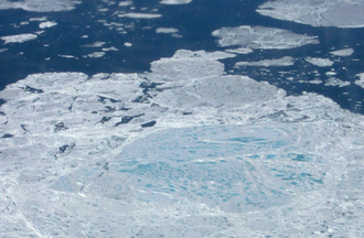
Aerial photograph showing a section of sea ice. The lighter blue areas are melt ponds and the darkest areas are open water; both have a lower albedo than the white sea ice. The melting ice contributes to ice–albedo feedback.

When ice melts, land or open water takes its place. Both land and open water are on average less reflective than ice and thus absorb more solar radiation. This causes more warming, which in turn causes more melting, and this cycle continues. During times of global cooling, additional ice increases the reflectivity which reduces the absorption of solar radiation which results in more cooling in a continuing cycle. Considered a faster feedback mechanism.

1870–2009 Northern hemisphere sea ice extent in million square kilometers. Blue shading indicates the pre-satellite era; data then is less reliable. In particular, the near-constant level extent in Autumn up to 1940 reflects lack of data rather than a real lack of variation.

Albedo change is also the main reason why IPCC predict polar temperatures in the northern hemisphere to rise up to twice as much as those of the rest of the world, in a process known as polar amplification. In September 2007, the Arctic sea ice area reached about half the size of the average summer minimum area between 1979 and 2000. Also in September 2007, Arctic sea ice retreated far enough for the Northwest Passage to become navigable to shipping for the first time in recorded history. The record losses of 2007 and 2008 may, however, be temporary. Mark Serreze of the US National Snow and Ice Data Center views 2030 as a "reasonable estimate" for when the summertime Arctic ice cap might be ice-free. The polar amplification of global warming is not predicted to occur in the southern hemisphere. The Antarctic sea ice reached its greatest extent on record since the beginning of observation in 1979, but the gain in ice in the south is exceeded by the loss in the north. The trend for global sea ice, northern hemisphere and southern hemisphere combined is clearly a decline.

Ice loss may have internal feedback processes, as melting of ice over land can cause eustatic sea level rise, potentially causing instability of ice shelves and inundating coastal ice masses, such as glacier tongues. Further, a potential feedback cycle exists due to earthquakes caused by isostatic rebound further destabilising ice shelves, glaciers and ice caps.

The ice–albedo in some sub-arctic forests is also changing, as stands of larch (which shed their needles in winter, allowing sunlight to reflect off the snow in spring and fall) are being replaced by spruce trees (which retain their dark needles all year).

Water vapor feedback

If the atmospheres are warmed, the saturation vapor pressure increases, and the amount of water vapor in the atmosphere will tend to increase. Since water vapor is a greenhouse gas, the increase in water vapor content makes the atmosphere warm further; this warming causes the atmosphere to hold still more water vapor (a positive feedback), and so on until other processes stop the feedback loop. The result is a much larger greenhouse effect than that due to CO₂ alone. Although this feedback process causes an increase in the absolute moisture content of the air, the relative humidity stays nearly constant or even decreases slightly because the air is warmer. Climate models incorporate this feedback. Water vapor feedback is strongly positive, with most evidence supporting a magnitude of 1.5 to 2.0 W/m²/K, sufficient to roughly double the warming that would otherwise occur. Water vapor feedback is considered a faster feedback mechanism.

Ocean-warming feedback

According to the U.S. National Oceanic and Atmospheric Administration: Ocean warming provides a good example of a potential positive feedback mechanism. The oceans are an important sink for CO2 through absorption of the gas into the water surface. As CO2 increases, it increases the warming potential of the atmosphere. If air temperatures warm, it should warm the oceans. The ability of the ocean to remove CO2 from the atmosphere decreases with increasing temperature. Because of this, increasing CO2 in the atmosphere could have effects that actually intensify the increase in CO2 in the atmosphere.

Negative

Blackbody radiation

As the temperature of a black body increases, the emission of infrared radiation back into space increases with the fourth power of its absolute temperature according to Stefan–Boltzmann law. This increases the amount of outgoing radiation as the Earth warms. The impact of this negative feedback effect is included in global climate models summarized by the IPCC. This is also called the Planck feedback.

Carbon cycle

Le Chatelier's principle

Following Le Chatelier's principle, the chemical equilibrium of the Earth's carbon cycle will shift in response to anthropogenic CO₂ emissions. The primary driver of this is the ocean, which absorbs anthropogenic CO₂ via the so-called solubility pump. At present this accounts for only about one third of the current emissions, but ultimately most (~75%) of the CO₂ emitted by human activities will dissolve in the ocean over a period of centuries: "A better approximation of the lifetime of fossil fuel CO₂ for public discussion might be 300 years, plus 25% that lasts forever". However, the rate at which the ocean will take it up in the future is less certain, and will be affected by stratification induced by warming and, potentially, changes in the ocean's thermohaline circulation.

Chemical weathering

Chemical weathering over the geological long term acts to remove CO₂ from the atmosphere. With current global warming, weathering is increasing, demonstrating significant feedbacks between climate and Earth surface. Biosequestration also captures and stores CO₂ by biological processes. The formation of shells by organisms in the ocean, over a very long time, removes CO₂ from the oceans. The complete conversion of CO₂ to limestone takes thousands to hundreds of thousands of years.

Net primary productivity

Net primary productivity changes in response to increased CO₂, as plants photosynthesis increased in response to increasing concentrations. However, this effect is swamped by other changes in the biosphere due to global warming.

Lapse rate

The atmosphere's temperature decreases with height in the troposphere. Since emission of infrared radiation varies with temperature, longwave radiation escaping to space from the relatively cold upper atmosphere is less than that emitted toward the ground from the lower atmosphere. Thus, the strength of the greenhouse effect depends on the atmosphere's rate of temperature decrease with height. Both theory and climate models indicate that global warming will reduce the rate of temperature decrease with height, producing a negative lapse rate feedback that weakens the greenhouse effect. However, in regions with strong inversions, such as the polar regions, the lapse rate feedback can be positive because the surface warms faster than higher altitudes, resulting in inefficient longwave cooling. Measurements of the rate of temperature change with height are very sensitive to small errors in observations, making it difficult to establish whether the models agree with observations.

Impacts on humans

Feedback loops from the book Al Gore (2006). An inconvenient truth.

The graphic suggests that the overall effect of climate change upon human numbers and development will be negative.

Climate sensitivity

From Wikipedia, the free encyclopedia

https://en.wikipedia.org/wiki/Climate_sensitivity

Diagram of factors that determine climate sensitivity. After increasing CO
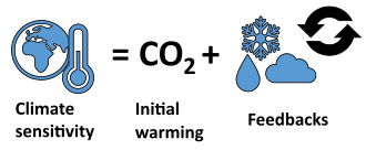
2 levels, there is an initial warming. This warming gets amplified by the net effect of feedbacks. Self-reinforcing feedbacks include the melting of sunlight-reflecting ice and higher evaporation increasing average atmospheric water vapour, which is a greenhouse gas.

Climate sensitivity is a measure of how much the Earth's climate will cool or warm after a change in the climate system, such as how much it will warm for doubling in carbon dioxide (CO
2) concentrations. In technical terms, climate sensitivity is the average change in the Earth's surface temperature in response to changes in radiative forcing, which is the difference between incoming and outgoing energy on Earth. Climate sensitivity is a key measure in climate science, and a focus area for climate scientists, who want to understand the ultimate consequences of anthroprogenic global warming.

The Earth's surface warms as a direct consequence of increased atmospheric CO
2, as well as increased concentrations of other greenhouse gases such as nitrous oxide and methane. The increasing temperatures have secondary effects on the climate system, such as an increase in atmospheric water vapour, which is itself also a greenhouse gas. Scientists do not know exactly how strong the climate feedbacks are and it is difficult to predict the precise amount of warming that will result from a given increase in greenhouse gas concentrations. If climate sensitivity turns out to be on the high side of scientific estimates, the Paris Agreement goal of limiting global warming to below 2 °C (3.6 °F) will be difficult to achieve.

The two primary types of climate sensitivity are the shorter-term "transient climate response", the increase in global average temperature that is expected to have occurred at a time when the atmospheric CO
2 concentration has doubled, and "equilibrium climate sensitivity", the higher long-term increase in global average temperature expected to occur after the effects of a doubled CO
2 concentration have had time to reach a steady state. Climate sensitivity is typically estimated in three ways: using direct observations of temperature and levels of greenhouse gases taken during the industrial age, using indirectly-estimated temperature and other measurements from the Earth's more distant past, and computer modelling the various aspects of the climate system with computers.

Background

The rate at which energy reaches Earth as sunlight and leaves Earth as heat radiation to space must balance, or the total amount of heat energy on the planet at any one time will rise or fall, which results in a planet that is warmer or cooler overall. An imbalance between the rates of incoming and outgoing radiation energy is called radiative forcing. A warmer planet radiates heat to space faster and so a new balance is eventually reached, with a higher planetary temperature. However, the warming of the planet also has knock-on effects, which create further warming in an exacerbating feedback loop. Climate sensitivity is a measure of how much temperature change a given amount of radiative forcing will cause.

Radiative forcing

Radiative forcing is generally defined as the imbalance between incoming and outgoing radiation at the top of the atmosphere. Radiative forcing is measured in Watts per square meter (W/m²), the average imbalance in energy per second for each square meter of the Earth's surface.

Changes to radiative forcing lead to long-term changes in global temperature. A number of factors can affect radiative forcing: increased downwelling radiation from the greenhouse effect, variability in solar radiation from changes in planetary orbit, changes in solar irradiance, direct and indirect effects caused by aerosols (for example changes in albedo from cloud cover), and changes in land use (deforestation or the loss of reflective ice cover). In contemporary research, radiative forcing by greenhouse gases is well understood. As of 2019, large uncertainties remain for aerosols.

Key numbers

Carbon dioxide (CO
2) levels rose from 280 parts per million (ppm) in the 18th century, when humans in the Industrial Revolution started burning significant amounts of fossil fuel such as coal, to over 415 ppm by 2020. As CO
2 is a greenhouse gas, it hinders heat energy from leaving the Earth's atmosphere. In 2016, atmospheric CO
2 levels had increased by 45% over preindustrial levels, and radiative forcing caused by increased CO
2 was already more than 50% higher than in pre-industrial times because of non-linear effects. Between the 18th-century start of the Industrial Revolution and the year 2020, the Earth's temperature rose by a little over one degree Celsius (about two degrees Fahrenheit).

Societal importance

Because the economics of climate change mitigation depend greatly on how quickly carbon neutrality needs to be achieved, climate sensitivity estimates can have important economic and policy-making implications. One study suggests that halving the uncertainty of the value for transient climate response (TCR) could save trillions of dollars. Scientists are uncertain about the precision of estimates of greenhouse gas increases on future temperature since a higher climate sensitivity would mean more dramatic increases in temperature, which makes it more prudent to take significant climate action. If climate sensitivity turns out to be on the high end of what scientists estimate, the Paris Agreement goal of limiting global warming to well below 2 °C cannot be achieved, and temperature increases will exceed that limit, at least temporarily. One study estimated that emissions cannot be reduced fast enough to meet the 2 °C goal if equilibrium climate sensitivity (the long-term measure) is higher than 3.4 °C (6.1 °F). The more sensitive the climate system is to changes in greenhouse gas concentrations, the more likely it is to have decades when temperatures are much higher or much lower than the longer-term average.

Contributors

Radiative forcing is one component of climate change. The radiative forcing caused by a doubling of atmospheric CO
2 levels (from the pre-industrial 280 ppm) is approximately 3.7 watts per square meter (W/m²). In the absence of feedbacks, the energy imbalance would eventually result in roughly 1 °C (1.8 °F) of global warming. That figure is straightforward to calculate by using the Stefan–Boltzmann lawand is undisputed.

A further contribution arises from climate feedback, both exacerbating and suppressing. The uncertainty in climate sensitivity estimates is entirely from the modelling of feedbacks in the climate system, including water vapour feedback, ice–albedo feedback, cloud feedback, and lapse rate feedback. Suppressing feedbacks tend to counteract warming by increasing the rate at which energy is radiated to space from a warmer planet. Exacerbating feedbacks increase warming; for example, higher temperatures can cause ice to melt, which reduces the ice area and the amount of sunlight the ice reflects, which in turn results in less heat energy being radiated back into space. Climate sensitivity depends on the balance between those feedbacks.

Measures

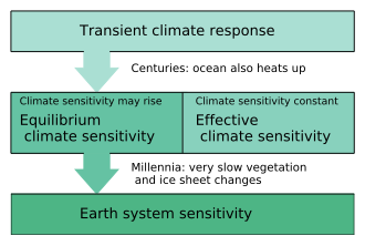
Schematic of how different measures of climate sensitivity relate to one another

Depending on the time scale, there are two main ways to define climate sensitivity: the short-term transient climate response (TCR) and the long-term equilibrium climate sensitivity (ECS), both of which incorporate the warming from exacerbating feedback loops. They are not discrete categories, but they overlap. Sensitivity to atmospheric CO
2 increases is measured in the amount of temperature change for doubling in the atmospheric CO
2 concentration.

Although the term "climate sensitivity" is usually used for the sensitivity to radiative forcing caused by rising atmospheric CO
2, it is a general property of the climate system. Other agents can also cause a radiative imbalance. Climate sensitivity is the change in surface air temperature per unit change in radiative forcing, and the climate sensitivity parameter is therefore expressed in units of °C/(W/m²). Climate sensitivity is approximately the same whatever the reason for the radiative forcing (such as from greenhouse gases or solar variation). When climate sensitivity is expressed as the temperature change for a level of atmospheric CO
2 double the pre-industrial level, its units are degrees Celsius (°C).

Transient climate response

The transient climate response (TCR) is defined as "is the change in the global mean surface temperature, averaged over a 20-year period, centered at the time of atmospheric carbon dioxide doubling, in a climate model simulation" in which the atmospheric CO
2 concentration increases at 1% per year. That estimate is generated by using shorter-term simulations. The transient response is lower than the equilibrium climate sensitivity because slower feedbacks, which exacerbate the temperature increase, take more time to respond in full to an increase in the atmospheric CO
2 concentration. For instance, the deep ocean takes many centuries to reach a new steady state after a perturbation during which it continues to serve as heatsink, which cools the upper ocean. The IPCC literature assessment estimates that the TCR likely lies between 1 °C (1.8 °F) and 2.5 °C (4.5 °F).

A related measure is the transient climate response to cumulative carbon emissions (TCRE), which is the globally averaged surface temperature change after 1000 GtC of CO
2 has been emitted. As such, it includes not only temperature feedbacks to forcing but also the carbon cycle and carbon cycle feedbacks.

Equilibrium climate sensitivity

The equilibrium climate sensitivity (ECS) is the long-term temperature rise (equilibrium global mean near-surface air temperature) that is expected to result from a doubling of the atmospheric CO
2 concentration (ΔT_2×). It is a prediction of the new global mean near-surface air temperature once the CO
2 concentration has stopped increasing, and most of the feedbacks have had time to have their full effect. Reaching an equilibrium temperature can take centuries or even millennia after CO
2 has doubled. ECS is higher than TCR because of the oceans' short-term buffering effects. Computer models are used for estimating the ECS. A comprehensive estimate means that modelling the whole time span during which significant feedbacks continue to change global temperatures in the model, such as fully-equilibrating ocean temperatures, requires running a computer model that covers thousands of years. There are, however, less computing-intensive methods.

The IPCC Sixth Assessment Report (AR6) stated that there is high confidence that ECS is within the range of 2.5°C to 4°C, with a best estimate of 3°C.

The long time scales involved with ECS make it arguably a less relevant measure for policy decisions around climate change.

Effective climate sensitivity

A common approximation to ECS is the effective equilibrium climate sensitivity, is an estimate of equilibrium climate sensitivity by using data from a climate system in model or real-world observations that is not yet in equilibrium. Estimates assume that the net amplification effect of feedbacks, as measured after some period of warming, will remain constant afterwards. That is not necessarily true, as feedbacks can change with time. In many climate models, feedbacks become stronger over time and so the effective climate sensitivity is lower than the real ECS.

Earth system sensitivity

By definition, equilibrium climate sensitivity does not include feedbacks that take millennia to emerge, such as long-term changes in Earth's albedo because of changes in ice sheets and vegetation. It includes the slow response of the deep oceans' warming, which also takes millennia, and so ECS fails to reflect the actual future warming that would occur if CO
2 is stabilized at double pre-industrial values. Earth system sensitivity (ESS) incorporates the effects of these slower feedback loops, such as the change in Earth's albedo from the melting of large continental ice sheets, wwhich covered much of the Northern Hemisphere during the Last Glacial Maximum and still cover Greenland and Antarctica). Changes in albedo as a result of changes in vegetation, as well as changes in ocean circulation, are also included. The longer-term feedback loops make the ESS larger than the ECS, possibly twice as large. Data from the geological history of Earth is used in estimating ESS. Differences between modern and long-ago climatic conditions mean that estimates of the future ESS are highly uncertain. Like for the ECS and the TCR, the carbon cycle is not included in the definition of the ESS, but all other elements of the climate system are included.

Sensitivity to nature of forcing

Different forcing agents, such as greenhouse gases and aerosols, can be compared using their radiative forcing, the initial radiative imbalance averaged over the entire globe. Climate sensitivity is the amount of warming per radiative forcing. To a first approximation, the cause of the radiative imbalance does not matter whether it is greenhouse gases or something else. However, radiative forcing from sources other than CO
2 can cause a somewhat larger or smaller surface warming than a similar radiative forcing from CO
2. The amount of feedback varies mainly because the forcings are not uniformly distributed over the globe. Forcings that initially warm the Northern Hemisphere, land, or polar regions are more strongly systematically effective at changing temperatures than an equivalent forcing from CO
2, which is more uniformly distributed over the globe. That is because those regions have more self-reinforcing feedbacks, such as the ice–albedo feedback. Several studies indicate that human-emitted aerosols are more effective than CO
2 at changing global temperatures, and volcanic forcing is less effective. When climate sensitivity to CO
2 forcing is estimated by using historical temperature and forcing (caused by a mix of aerosols and greenhouse gases), and that effect is not taken into account, climate sensitivity is underestimated.

State dependence

Artist impression of a Snowball Earth.

Climate sensitivity has been defined as the short- or long-term temperature change resulting from any doubling of CO
2, but there is evidence that the sensitivity of Earth's climate system is not constant. For instance, the planet has polar ice and high-altitude glaciers. Until the world's ice has completely melted, an exacerbating ice–albedo feedback loop makes the system more sensitive overall. Throughout Earth's history, multiple periods are thought to have snow and ice cover almost the entire globe. In most models of "Snowball Earth,", parts of the tropics were at least intermittently free of ice cover. As the ice advanced or retreated, climate sensitivity must have been very high, as the large changes in area of ice cover would have made for a very strong ice–albedo feedback. Volcanic atmospheric composition changes are thought to have provided the radiative forcing needed to escape the snowball state.

Equilibrium climate sensitivity can change with climate.

Throughout the Quaternary period (the most recent 2.58 million years), climate has oscillated between glacial periods, the most recent one being the Last Glacial Maximum, and interglacial periods, the most recent one being the current Holocene, but the period's climate sensitivity is difficult to determine. The Paleocene–Eocene Thermal Maximum, about 55.5 million years ago, was unusually warm and may have been characterized by above-average climate sensitivity.

Climate sensitivity may further change if tipping points are crossed. It is unlikely that tipping points will cause short-term changes in climate sensitivity. If a tipping point is crossed, climate sensitivity is expected to change at the time scale of the subsystem that hits its tipping point. Especially if there are multiple interacting tipping points, the transition of climate to a new state may be difficult to reverse.

The two most common definitions of climate sensitivity specify the climate state: the ECS and the TCR are defined for a doubling with respect to the CO
2 levels in the pre-industrial era. Because of potential changes in climate sensitivity, the climate system may warm by a different amount after a second doubling of CO
2 from after a first doubling. The effect of any change in climate sensitivity is expected to be small or negligible in the first century after additional CO
2 is released into the atmosphere.

Estimates

Historical estimates

Svante Arrhenius in the 19th century was the first person to quantify global warming as a consequence of a doubling of the concentration of CO
2. In his first paper on the matter, he estimated that global temperature would rise by around 5 to 6 °C (9.0 to 10.8 °F) if the quantity of CO
2 was doubled. In later work, he revised that estimate to 4 °C (7.2 °F). Arrhenius used Samuel Pierpont Langley's observations of radiation emitted by the full moon to estimate the amount of radiation that was absorbed by water vapour and by CO
2. To account for water vapour feedback, he assumed that relative humidity would stay the same under global warming.

The first calculation of climate sensitivity that used detailed measurements of absorption spectra, as well as the first calculation to use a computer for numerical integration of the radiative transfer through the atmosphere, was performed by Syukuro Manabe and Richard Wetherald in 1967. Assuming constant humidity, they computed an equilibrium climate sensitivity of 2.3 °C per doubling of CO
2, which they rounded to 2 °C, the value most often quoted from their work, in the abstract of the paper. The work has been called "arguably the greatest climate-science paper of all time" and "the most influential study of climate of all time."

A committee on anthropogenic global warming, convened in 1979 by the United States National Academy of Sciences and chaired by Jule Charney, estimated equilibrium climate sensitivity to be 3 °C (5.4 °F), plus or minus 1.5 °C (2.7 °F). The Manabe and Wetherald estimate (2 °C (3.6 °F)), James E. Hansen's estimate of 4 °C (7.2 °F), and Charney's model were the only models available in 1979. According to Manabe, speaking in 2004, "Charney chose 0.5 °C as a reasonable margin of error, subtracted it from Manabe's number, and added it to Hansen's, giving rise to the 1.5 to 4.5 °C (2.7 to 8.1 °F) range of likely climate sensitivity that has appeared in every greenhouse assessment since ...." In 2008, climatologist Stefan Rahmstorf said: "At that time [it was published], the [Charney report estimate's] range [of uncertainty] was on very shaky ground. Since then, many vastly improved models have been developed by a number of climate research centers around the world."

Intergovernmental Panel on Climate Change

Historical estimates of climate sensitivity from the IPCC assessments. The first three reports gave a qualitative likely range, and the fourth and the fifth assessment report formally quantified the uncertainty. The dark blue range is judged as being more than 66% likely.

Despite considerable progress in the understanding of Earth's climate system, assessments continued to report similar uncertainty ranges for climate sensitivity for some time after the 1979 Charney report. The 1990 IPCC First Assessment Report estimated that equilibrium climate sensitivity to a doubling of CO
2 lay between 1.5 and 4.5 °C (2.7 and 8.1 °F), with a "best guess in the light of current knowledge" of 2.5 °C (4.5 °F). The report used models with simplified representations of ocean dynamics. The IPCC supplementary report, 1992, which used full-ocean circulation models, saw "no compelling reason to warrant changing" the 1990 estimate and the IPCC Second Assessment Report stated, "No strong reasons have emerged to change [these estimates]," In the reports, much of the uncertainty around climate sensitivity was attributed to insufficient knowledge of cloud processes. The 2001 IPCC Third Assessment Report also retained this likely range.

Authors of the 2007 IPCC Fourth Assessment Report stated that confidence in estimates of equilibrium climate sensitivity had increased substantially since the Third Annual Report. The IPCC authors concluded that ECS is very likely to be greater than 1.5 °C (2.7 °F) and likely to lie in the range 2 to 4.5 °C (3.6 to 8.1 °F), with a most likely value of about 3 °C (5.4 °F). The IPCC stated that fundamental physical reasons and data limitations prevent a climate sensitivity higher than 4.5 °C (8.1 °F) from being ruled out, but the climate sensitivity estimates in the likely range agreed better with observations and the proxy climate data.

The 2013 IPCC Fifth Assessment Report reverted to the earlier range of 1.5 to 4.5 °C (2.7 to 8.1 °F) (with high confidence), because some estimates using industrial-age data came out low. (See the next section for details.) The report also stated that ECS is extremely unlikely to be less than 1 °C (1.8 °F) (high confidence), and it is very unlikely to be greater than 6 °C (11 °F) (medium confidence). Those values were estimated by combining the available data with expert judgement.

When the IPCC began to produce its IPCC Sixth Assessment Report, many climate models began to show a higher climate sensitivity. The estimates for Equilibrium Climate Sensitivity changed from 3.2 °C to 3.7 °C and the estimates for the Transient climate response from 1.8 °C, to 2.0 °C. That is probably because of better understanding of the role of clouds and aerosols.

Methods of estimation

Using Industrial Age (1750–present) data

Climate sensitivity can be estimated using the observed temperature increase, the observed ocean heat uptake, and the modelled or observed radiative forcing. The data are linked through a simple energy-balance model to calculate climate sensitivity. Radiative forcing is often modelled because Earth observation satellites measuring it has existed during only part of the Industrial Age (only since the mid-20th century). Estimates of climate sensitivity calculated by using these global energy constraints have consistently been lower than those calculated by using other methods, around 2 °C (3.6 °F) or lower.

Estimates of transient climate response (TCR) that have been calculated from models and observational data can be reconciled if it is taken into account that fewer temperature measurements are taken in the polar regions, which warm more quickly than the Earth as a whole. If only regions for which measurements are available are used in evaluating the model, the differences in TCR estimates are negligible.

A very simple climate model could estimate climate sensitivity from Industrial Age data by waiting for the climate system to reach equilibrium and then by measuring the resulting warming, $Δ T eq$ (°C). Computation of the equilibrium climate sensitivity, S (°C), using the radiative forcing $Δ F$ (W/m²) and the measured temperature rise, would then be possible. The radiative forcing resulting from a doubling of CO
2, $\times$ , is relatively well known, at about 3.7 W/m². Combining that information results in this equation:

S=\Delta T_{eq}\times F_{2\times CO_{2}}/\Delta F

However, the climate system is not in equilibrium since the actual warming lags the equilibrium warming, largely because the oceans take up heat and will take centuries or millennia to reach equilibrium. Estimating climate sensitivity from Industrial Age data requires an adjustment to the equation above. The actual forcing felt by the atmosphere is the radiative forcing minus the ocean's heat uptake, $H$ (W/m²) and so climate sensitivity can be estimated:

S=\Delta T\times F_{2\times CO_{2}}/(\Delta F-H).

The global temperature increase between the beginning of the Industrial Period, which is (taken as 1750, and 2011 was about 0.85 °C (1.53 °F). In 2011, the radiative forcing from CO
2 and other long-lived greenhouse gases (mainly methane, nitrous oxide, and chlorofluorocarbon) that have been emitted since the 18th century was roughly 2.8 W/m². The climate forcing, $Δ F$ , also contains contributions from solar activity (+0.05 W/m²), aerosols (−0.9 W/m²), ozone (+0.35 W/m²), and other smaller influences, which brings the total forcing over the Industrial Period to 2.2 W/m², according to the best estimate of the IPCC AR5, with substantial uncertainty. The ocean heat uptake estimated by the IPCC AR5 as 0.42 W/m², yields a value for S of 1.8 °C (3.2 °F).

Other strategies

In theory, Industrial Age temperatures could also be used to determine a time scale for the temperature response of the climate system and thus climate sensitivity: if the effective heat capacity of the climate system is known, and the timescale is estimated using autocorrelation of the measured temperature, an estimate of climate sensitivity can be derived. In practice, however, the simultaneous determination of the time scale and heat capacity is difficult.

Attempts have been made to use the 11-year solar cycle to constrain the transient climate response. Solar irradiance is about 0.9 W/m² higher during a solar maximum than during a solar minimum, and those effect can be observed in measured average global temperatures from 1959 to 2004. Unfortunately, the solar minima in the period coincided with volcanic eruptions, which have a cooling effect on the global temperature. Because the eruptions caused a larger and less well-quantified decrease in radiative forcing than the reduced solar irradiance, it is questionable whether useful quantitative conclusions can be derived from the observed temperature variations.

Observations of volcanic eruptions have also been used to try to estimate climate sensitivity, but as the aerosols from a single eruption last at most a couple of years in the atmosphere, the climate system can never come close to equilibrium, and there is less cooling than there would be if the aerosols stayed in the atmosphere for longer. Therefore, volcanic eruptions give information only about a lower bound on transient climate sensitivity.

Using data from Earth's past

Historical climate sensitivity can be estimated by using reconstructions of Earth's past temperatures and CO
2 levels. Paleoclimatologists have studied different geological periods, such as the warm Pliocene (5.3 to 2.6 million years ago) and the colder Pleistocene (2.6 million to 11,700 years ago), and sought periods that are in some way analogous to or informative about current climate change. Climates further back in Earth's history are more difficult to study because fewer data are available about them. For instance, past CO
2 concentrations can be derived from air trapped in ice cores, but as of 2020, the oldest continuous ice core is less than one million years old. Recent periods, such as the Last Glacial Maximum (LGM) (about 21,000 years ago) and the Mid-Holocene (about 6,000 years ago), are often studied, especially when more information about them becomes available.

A 2007 estimate of sensitivity made using data from the most recent 420 million years is consistent with sensitivities of current climate models and with other determinations. The Paleocene–Eocene Thermal Maximum (about 55.5 million years ago), a 20,000-year period during which massive amount of carbon entered the atmosphere and average global temperatures increased by approximately 6 °C (11 °F), also provides a good opportunity to study the climate system when it was in a warm state. Studies of the last 800,000 years have concluded that climate sensitivity was greater in glacial periods than in interglacial periods.

As the name suggests, the Last Glacial Maximum was much colder than today, and good data on atmospheric CO
2 concentrations and radiative forcing from that period are available. The period's orbital forcing was different from today's but had little effect on mean annual temperatures. Estimating climate sensitivity from the Last Glacial Maximum can be done by several different ways. One way is to use estimates of global radiative forcing and temperature directly. The set of feedback mechanisms active during the period, however, may be different from the feedbacks caused by a present doubling of CO
2, which introduces additional uncertainty. In a different approach, a model of intermediate complexity is used to simulate conditions during the period. Several versions of this single model are run, with different values chosen for uncertain parameters, such that each version has a different ECS. Outcomes that best simulate the LGM's observed cooling probably produce the most realistic ECS values.

Using climate models

Frequency distribution of equilibrium climate sensitivity based on simulations of the doubling of CO
2. Each model simulation has different estimates for processes, which scientists do not sufficiently understand. Few of the simulations result in less than 2 °C (3.6 °F) of warming or significantly more than 4 °C (7.2 °F). However, the positive skew, which is also found in other studies, suggests that if carbon dioxide concentrations double, the probability of large or very large increases in temperature is greater than the probability of small increases.

Climate models simulate the CO
2-driven warming of the future as well as the past. They operate on principles similar to those underlying models that predict the weather, but they focus on longer-term processes. Climate models typically begin with a starting state and then apply physical laws and knowledge about biology to generate subsequent states. As with weather modelling, no computer has the power to model the complexity of the entire planet and so simplifications are used to reduce that complexity to something manageable. An important simplification divides Earth's atmosphere into model cells. For instance, the atmosphere might be divided into cubes of air ten or one hundred kilometers on a side. Each model cell is treated as if it were homogeneous. Calculations for model cells are much faster than trying to simulate each molecule of air separately.

A lower model resolution (large model cells and long time steps) takes less computing power but cannot simulate the atmosphere in as much detail. A model cannot simulate processes smaller than the model cells or shorter-term than a single time step. The effects of the smaller-scale and shorter-term processes must therefore be estimated by using other methods. Physical laws contained in the models may also be simplified to speed up calculations. The biosphere must be included in climate models. The effects of the biosphere are estimated by using data on the average behaviour of the average plant assemblage of an area under the modelled conditions. Climate sensitivity is therefore an emergent property of these models. It is not prescribed, but it follows from the interaction of all the modelled processes.

To estimate climate sensitivity, a model is run by using a variety of radiative forcings (doubling quickly, doubling gradually, or following historical emissions) and the temperature results are compared to the forcing applied. Different models give different estimates of climate sensitivity, but they tend to fall within a similar range, as described above.

Testing, comparisons, and estimates

Modelling of the climate system can lead to a wide range of outcomes. Models are often run that use different plausible parameters in their approximation of physical laws and the behaviour of the biosphere, which forms a perturbed physics ensemble, which attempts attempts to model the sensitivity of the climate to different types and amounts of change in each parameter. Alternatively, structurally-different models developed at different institutions are put together, creating an ensemble. By selecting only the simulations that can simulate some part of the historical climate well, a constrained estimate of climate sensitivity can be made. One strategy for obtaining more accurate results is placing more emphasis on climate models that perform well in general.

A model is tested using observations, paleoclimate data, or both to see if it replicates them accurately. If it does not, inaccuracies in the physical model and parametrizations are sought, and the model is modified. For models used to estimate climate sensitivity, specific test metrics that are directly and physically linked to climate sensitivity are sought. Examples of such metrics are the global patterns of warming, the ability of a model to reproduce observed relative humidity in the tropics and subtropics, patterns of heat radiation, and the variability of temperature around long-term historical warming. Ensemble climate models developed at different institutions tend to produce constrained estimates of ECS that are slightly higher than 3 °C (5.4 °F). The models with ECS slightly above 3 °C (5.4 °F) simulate the above situations better than models with a lower climate sensitivity.

Many projects and groups exist to compare and to analyse the results of multiple models. For instance, the Coupled Model Intercomparison Project (CMIP) has been running since the 1990s.

In preparation for the 2021 IPCC Sixth Assessment Report, a new generation of climate models have been developed by scientific groups around the world. The average estimated climate sensitivity has increased in Coupled Model Intercomparison Project Phase 6 (CMIP6) compared to the previous generation, with values spanning 1.8 to 5.6 °C (3.2 to 10.1 °F) across 27 global climate models and exceeding 4.5 °C (8.1 °F) in 10 of them. The cause of the increased ECS lies mainly in improved modelling of clouds. Temperature rises are now believed to cause sharper decreases in the number of low clouds, and fewer low clouds means more sunlight is absorbed by the planet and less reflected to space. Models with the highest ECS values, however, are not consistent with observed warming.

Search This Blog