An integer programming problem is a mathematical optimization or feasibility program in which some or all of the variables are restricted to be integers. In many settings the term refers to integer linear programming (ILP), in which the objective function and the constraints (other than the integer constraints) are linear.
Integer programming is NP-complete. In particular, the special case of 0-1 integer linear programming, in which unknowns are binary, and only the restrictions must be satisfied, is one of Karp's 21 NP-complete problems.
If some decision variables are not discrete, the problem is known as a mixed-integer programming problem.
Canonical and standard form for ILPs
In integer linear programming, the canonical form is distinct from the standard form. An integer linear program in canonical form is expressed thus (note that it is the vector which is to be decided):
and an ILP in standard form is expressed as
where are vectors and is a matrix. As with linear programs, ILPs not in standard form can be converted to standard form by eliminating inequalities, introducing slack variables () and replacing variables that are not sign-constrained with the difference of two sign-constrained variables
Example
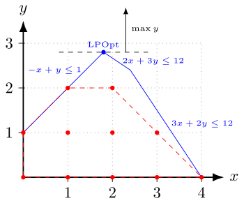
The plot above shows the following problem.
The feasible integer points are shown in red, and the red dashed lines indicate their convex hull, which is the smallest convex polyhedron that contains all of these points. The blue lines together with the coordinate axes define the polyhedron of the LP relaxation, which is given by the inequalities without the integrality constraint. The goal of the optimization is to move the black dashed line as far upward while still touching the polyhedron. The optimal solutions of the integer problem are the points and which both have an objective value of 2. The unique optimum of the relaxation is with objective value of 2.8. If the solution of the relaxation is rounded to the nearest integers, it is not feasible for the ILP.
Proof of NP-hardness
The following is a reduction from minimum vertex cover to integer programming that will serve as the proof of NP-hardness.
Let be an undirected graph. Define a linear program as follows:
Given that the constraints limit to either 0 or 1, any feasible solution to the integer program is a subset of vertices. The first constraint implies that at least one end point of every edge is included in this subset. Therefore, the solution describes a vertex cover. Additionally given some vertex cover C, can be set to 1 for any and to 0 for any thus giving us a feasible solution to the integer program. Thus we can conclude that if we minimize the sum of we have also found the minimum vertex cover.
Variants
Mixed-integer linear programming (MILP) involves problems in which only some of the variables, , are constrained to be integers, while other variables are allowed to be non-integers.
Zero-one linear programming (or binary integer programming) involves problems in which the variables are restricted to be either 0 or 1. Any bounded integer variable can be expressed as a combination of binary variables. For example, given an integer variable, , the variable can be expressed using binary variables:
Applications
There are two main reasons for using integer variables when modeling problems as a linear program:
- The integer variables represent quantities that can only be integer. For example, it is not possible to build 3.7 cars.
- The integer variables represent decisions (e.g. whether to include an edge in a graph) and so should only take on the value 0 or 1.
These considerations occur frequently in practice and so integer linear programming can be used in many applications areas, some of which are briefly described below.
Production planning
Mixed-integer programming has many applications in industrial productions, including job-shop modelling. One important example happens in agricultural production planning involves determining production yield for several crops that can share resources (e.g. Land, labor, capital, seeds, fertilizer, etc.). A possible objective is to maximize the total production, without exceeding the available resources. In some cases, this can be expressed in terms of a linear program, but the variables must be constrained to be integer.
Scheduling
These problems involve service and vehicle scheduling in transportation networks. For example, a problem may involve assigning buses or subways to individual routes so that a timetable can be met, and also to equip them with drivers. Here binary decision variables indicate whether a bus or subway is assigned to a route and whether a driver is assigned to a particular train or subway. The zero-one programming technique has been successfully applied to solve a project selection problem in which projects are mutually exclusive and/or technologically interdependent. It is used in a special case of integer programming, in which all the decision variables are integers. It can assume the values either as zero or one.
Territorial partitioning
Territorial partitioning or districting problem consists in partitioning a geographical region into districts in order to plan some operations while considering different criteria or constraints. Some requirements for this problem are: contiguity, compactness, balance or equity, respect of natural boundaries, and socio-economic homogeneity. Some applications for this type of problem include: political districting, school districting, health services districting and waste management districting.
Telecommunications networks
The goal of these problems is to design a network of lines to install so that a predefined set of communication requirements are met and the total cost of the network is minimal. This requires optimizing both the topology of the network along with the setting the capacities of the various lines. In many cases, the capacities are constrained to be integer quantities. Usually there are, depending on the technology used, additional restrictions that can be modeled as linear inequalities with integer or binary variables.
Cellular networks
The task of frequency planning in GSM mobile networks involves distributing available frequencies across the antennas so that users can be served and interference is minimized between the antennas. This problem can be formulated as an integer linear program in which binary variables indicate whether a frequency is assigned to an antenna.
Other applications
- Cash flow matching
- Energy system optimization
- UAV guidance
Algorithms
The naive way to solve an ILP is to simply remove the constraint that x is integer, solve the corresponding LP (called the LP relaxation of the ILP), and then round the entries of the solution to the LP relaxation. But, not only may this solution not be optimal, it may not even be feasible; that is, it may violate some constraint.
Using total unimodularity
While in general the solution to LP relaxation will not be guaranteed to be integral, if the ILP has the form such that where and have all integer entries and is totally unimodular, then every basic feasible solution is integral. Consequently, the solution returned by the simplex algorithm is guaranteed to be integral. To show that every basic feasible solution is integral, let be an arbitrary basic feasible solution . Since is feasible, we know that . Let be the elements corresponding to the basis columns for the basic solution . By definition of a basis, there is some square submatrix of with linearly independent columns such that .
Since the columns of are linearly independent and is square, is nonsingular, and therefore by assumption, is unimodular and so . Also, since is nonsingular, it is invertible and therefore . By definition, . Here denotes the adjugate of and is integral because is integral. Therefore,
Thus, if the matrix of an ILP is totally unimodular, rather than use an ILP algorithm, the simplex method can be used to solve the LP relaxation and the solution will be integer.
Exact algorithms
When the matrix is not totally unimodular, there are a variety of algorithms that can be used to solve integer linear programs exactly. One class of algorithms are cutting plane methods which work by solving the LP relaxation and then adding linear constraints that drive the solution towards being integer without excluding any integer feasible points.
Another class of algorithms are variants of the branch and bound method. For example, the branch and cut method that combines both branch and bound and cutting plane methods. Branch and bound algorithms have a number of advantages over algorithms that only use cutting planes. One advantage is that the algorithms can be terminated early and as long as at least one integral solution has been found, a feasible, although not necessarily optimal, solution can be returned. Further, the solutions of the LP relaxations can be used to provide a worst-case estimate of how far from optimality the returned solution is. Finally, branch and bound methods can be used to return multiple optimal solutions.
Exact algorithms for a small number of variables
Suppose is an m-by-n integer matrix and is an m-by-1 integer vector. We focus on the feasibility problem, which is to decide whether there exists an n-by-1 vector satisfying .
Let V be the maximum absolute value of the coefficients in and . If n (the number of variables) is a fixed constant, then the feasibility problem can be solved in time polynomial in m and log V. This is trivial for the case n=1. The case n=2 was solved in 1981 by Herbert Scarf.[11] The general case was solved in 1983 by Hendrik Lenstra, combining ideas by László Lovász and Peter van Emde Boas.[12]
In the special case of 0-1 ILP, Lenstra's algorithm is equivalent to complete enumeration: the number of all possible solutions is fixed (2n), and checking the feasibility of each solution can be done in time poly(m, log V). In the general case, where each variable can be an arbitrary integer, complete enumeration is impossible. Here, Lenstra's algorithm uses ideas from Geometry of numbers. It transforms the original problem into an equivalent one with the following property: either the existence of a solution is obvious, or the value of (the n-th variable) belongs to an interval whose length is bounded by a function of n. In the latter case, the problem is reduced to a bounded number of lower-dimensional problems. The run-time complexity of the algorithm has been improved in several steps:
- The original algorithm of Lenstra had run-time .
- Kannan presented an improved algorithm with run-time .
- Frank and Tardos presented a different improved algorithm. The improved runtime is , where is the number of input bits, which is in in which n is varying but m (the number of constraints) is constant.
Heuristic methods
Since integer linear programming is NP-hard, many problem instances are intractable and so heuristic methods must be used instead. For example, tabu search can be used to search for solutions to ILPs. To use tabu search to solve ILPs, moves can be defined as incrementing or decrementing an integer constrained variable of a feasible solution while keeping all other integer-constrained variables constant. The unrestricted variables are then solved for. Short-term memory can consist of previously tried solutions while medium-term memory can consist of values for the integer constrained variables that have resulted in high objective values (assuming the ILP is a maximization problem). Finally, long-term memory can guide the search towards integer values that have not previously been tried.
Other heuristic methods that can be applied to ILPs include
- Hill climbing
- Simulated annealing
- Reactive search optimization
- Ant colony optimization
- Hopfield neural networks
There are also a variety of other problem-specific heuristics, such as the k-opt heuristic for the traveling salesman problem. A disadvantage of heuristic methods is that if they fail to find a solution, it cannot be determined whether it is because there is no feasible solution or whether the algorithm simply was unable to find one. Further, it is usually impossible to quantify how close to optimal a solution returned by these methods are.


![\mathbf {x} _{0}=[x_{n_{1}},x_{n_{2}},\cdots ,x_{n_{j}}]](https://wikimedia.org/api/rest_v1/media/math/render/svg/dfa84a77e8f9f05bb2dcbda53c5b400f8e899adf)


