Recurrent laryngeal nerve -- evidence forevolution

From Wikipedia, the free encyclopedia

Recurrent laryngeal nerve
Course of the left recurrent laryngeal nerve
Posterior view of tracheal and bronchial lymph glands, with the left and right recurrent nerves visible on either side.
Details
Latin	nervus laryngeus recurrens
From	vagus nerve
Innervates	larynx posterior cricoarytenoid lateral cricoarytenoid arytenoid thyroarytenoid aryepiglottis esophagus
Identifiers
Gray's	p.912
Dorlands /Elsevier	n_05/12566073
TA	A14.2.01.166
FMA	6246
Anatomical terms of neuroanatomy

The recurrent laryngeal nerve (RLN) is a branch of the vagus nerve (cranial nerve X) that supplies all the intrinsic muscles of the larynx, with the exception of the cricothyroid muscles. There are two recurrent laryngeal nerves, right and left, in the human body. The nerves emerge from the vagus nerve at the level of the arch of aorta, and then travel up the side of the trachea to the larynx. The right and left nerves are not symmetrical, with the left nerve looping under the aortic arch, and the right nerve looping under the right subclavian artery then traveling upwards. Additionally, the nerves are one of few nerves that follow a recurrent course, moving in the opposite direction to the nerve they branch from, a fact from which they gain their name.

The recurrent laryngeal nerves supply sensation to the larynx below the vocal cords, gives cardiac branches to the deep cardiac plexus, and branches to the trachea, esophagus and the inferior constrictor muscles. The posterior cricoarytenoid muscles, the only muscles that can open the vocal cords, are innervated by this nerve.

The recurrent laryngeal nerves are the nerves of the sixth pharyngeal arch. The existence of the recurrent laryngeal nerve was first documented by the physician Galen.

Structure

Passing under the subclavian artery, the right recurrent laryngeal nerve has a much shorter course than the left which passes under the aortic arch and ligamentum arteriosum.

The recurrent laryngeal nerves branch from the vagus nerve, relative to which they get their names; the term "recurrent" from Latin: re- (back) and currere (to run),^[1] indicates they run in the opposite direction to the vagus nerves from which they branch.^[2] The vagus nerves run down into the thorax, and the recurrent laryngeal nerves run up to the larynx.^{[3]:930–931}

The vagus nerves, from which the recurrent laryngeal nerves branch, exit the skull at the jugular foramen and travel within the carotid sheath alongside the carotid arteries through the neck. The recurrent laryngeal nerves branch off the vagus, the left at the aortic arch, and the right at the right subclavian artery. The left RLN passes in front of the arch, and then wraps underneath and behind it. After branching, the nerves typically ascend in a groove at the junction of the trachea and esophagus.^{[4]:1346–1347} They then pass behind the posterior, middle part of the outer lobes of the thyroid gland and enter the larynx underneath the inferior constrictor muscle,^[3]:918 passing through the thyrohyoid membrane.^[5] The terminal branch is called the inferior laryngeal nerve.^[6]:19

Unlike the other nerves supplying the larynx, the right and left RLNs lack bilateral symmetry.^[7] The left RLN is longer than the right, because it crosses under the arch of the aorta at the ligamentum arteriosum.^{[4]:1346–1347}

Nucleus

The somatic motor fibers that innervate the laryngeal and pharyngeal muscles are located in the nucleus ambiguous and emerge from the medulla in the cranial root of the accessory nerve. Fibers cross over to and join the vagus nerve in the jugular foramen.^[8]:86–88 Sensory cell bodies are located in the inferior jugular ganglion,^[9] and the fibers terminate in the solitary nucleus.^[8]:86–88 Parasympathetic fibers to segments of the trachea and esophagus in the neck originate in the dorsal nucleus of the vagus nerve.^[9]

Development

During human and all vertebrate development, a series of pharyngeal arch pairs form in the developing embryo. These project forward from the back of the embryo towards the front of the face and neck. Each arch develops its own artery, nerve that controls a distinct muscle group, and skeletal tissue. The arches are numbered from 1 to 6, with 1 being the arch closest to the head of the embryo, and the fifth arch only existing transiently.^{[10]:318–323}

Arches 4 and 6 produce the laryngeal cartilages. The nerve of the sixth arch becomes the recurrent laryngeal nerve. The nerve of the fourth arch gives rise to the superior laryngeal nerve. The arteries of the fourth arch, which project between the nerves of the fourth and sixth arches, become the left-sided arch of the aorta and the right subclavian artery. The arteries of the sixth arch persists as the ductus arteriosus on the left, and is obliterated on the right.^{[10]:318–323}

After birth, the ductus arteriosus regresses to form the ligamentum arteriosum. During growth, these arteries descend into their ultimate positions in the chest, creating the elongated recurrent paths.^{[10]:318–323}

Variation

In roughly 1 out of every 100–200 people, the right inferior laryngeal nerve is nonrecurrent, branching off the vagus nerve around the level of the cricoid cartilage. Typically, such a configuration is accompanied by variation in the arrangement of the major arteries in the chest; most commonly, the right subclavian artery arises from the left side of the aorta and crosses behind the esophagus. A left nonrecurrent inferior laryngeal nerve is even more uncommon, requiring the aortic arch be on the right side, accompanied by an arterial variant which prevents the nerve from being drawn into the chest by the left subclavian.^{[11]:10, 48}

In about four people out of five, there is a connecting branch between the inferior laryngeal nerve, a branch of the RLN, and the internal laryngeal nerve, a branch of the superior laryngeal nerve. This is commonly called the anastomosis of Galen (Latin: ansa galeni), even though anastamosis usually refers to a blood vessel,^[12][13]:35 and is one of several documented anastamosis between the two nerves.^[14]

As the recurrent nerve hooks around the subclavian artery or aorta, it gives off several branches. There is suspected variability in the configuration of these branches to the cardiac plexus, trachea, esophagus and inferior pharyngeal constrictor muscle.^[15]

Function

The recurrent laryngeal nerves control all intrinsic muscles of the larynx except for the cricothyroid muscle.^[15][a] These muscles act to open and close the vocal cords, and include the posterior cricoarytenoid muscles, the only muscle to open the vocal cords.^[16]:10–11 The nerves supply muscles on the same side of the body, with the exception of the interarytenoid muscle, which is innervated from both sides.^[15]

The nerves also carry sensory information from the mucous membranes of the larynx below the lower surface of the vocal fold,^[17]:847–9 as well as sensory, secretory and motor fibres to the cervical segments of the esophagus and the trachea.^{[8]:142–144}

Clinical significance

Injury

Recurrent laryngeal nerve visible during resection of a goitre

The recurrent laryngeal nerves may be injured as a result of trauma, during surgery, as a result of tumour spread, or due to other means.^[16]:12 Injury to the recurrent laryngeal nerves can result in a weakened voice (hoarseness) or loss of voice (aphonia) and cause problems in the respiratory tract.^[16]:11–12 Injury to the nerve may paralyze the posterior cricoarytenoid muscle on the same side. This is the sole muscle responsible for opening the vocal cords, and paralysis may cause difficulty breathing (dyspnea) during physical activity.^[18] Injury to both the right and left nerve may result in more serious damage, such as the inability to speak. Additional problems may emerge during healing, as nerve fibres that re-anastamose may result in vocal cord motion impairment, uncoordinated movements of the vocal cord.^[16]:12–13

Surgery

The nerve receives close attention from surgeons since during neck surgery, especially thyroid and parathyroid surgery, the nerve is at risk for injury.^[4] Nerve damage can be assessed by laryngoscopy, during which a stroboscopic light confirms the absence of movement in the affected side of the vocal cords. The right recurrent laryngeal nerve is more susceptible to damage during thyroid surgery because it is close to the bifurcation of the right inferior thyroid artery, variably passing in front of, behind, or between the branches.^[17]:820–1 The nerve is permanently damaged in 0.3–3% of thyroid surgery, and transiently in 3–8% of surgeries, and is one of the leading causes of medicolegal issues for surgeons.^[19]

Tumors

The RLN may be compressed by tumors. Studies have shown that 2–18% of lung cancer patients develop hoarseness because of recurrent laryngeal nerve compression, usually left-sided.^[20] This is associated with worse outcomes, and when found as a presenting symptom, often indicates inoperable tumors. The nerve may be severed intentionally during lung cancer surgery in order to fully remove a tumor.^[21]:330

Other disease

In Ortner's syndrome or cardiovocal syndrome, a rare cause of left recurrent laryngeal nerve palsy, expansion of structures within the heart or major blood vessels impinges upon the nerve, causing symptoms of unilateral nerve injury.^[22]

Other animals

Horses are subject to equine recurrent laryngeal neuropathy, a disease of the axons of the recurrent laryngeal nerves. The cause is not known, although a genetic predisposition is suspected. The length of the nerve is a factor since it is more common in larger horses, and the left side is affected almost exclusively. As the nerve cells die, there is a progressive paralysis of the larynx, causing the airway to collapse. The common presentation is a sound, ranging from a musical whistle to a harsh roar or heaving gasping noise (stertorous), accompanied by worsening performance. The condition is incurable, but surgery can keep the airway open. Experiments with nerve grafts have been tried.^{[23]:421–426}

Although uncommon in dogs, bilateral recurrent laryngeal nerve disease may be the cause of wheezing (stridor) when middle-aged dogs inhale.^[24]:771

In sauropod dinosaurs, the vertebrates with the longest necks, the total length of the vagus nerve and recurrent laryngeal nerve would have been up to 28 metres (92 ft) long in Supersaurus, but this would not the longest neuron that ever existed, since some neurons reaching the tip of the tail would have exceeded 30 metres (98 ft).^[25]

Evidence of evolution

The extreme detour of the recurrent laryngeal nerves, about 4.6 metres (15 ft) in the case of giraffes,^[26]:74–75 is cited as evidence of evolution. The nerve's route would have been direct in the fish-like ancestors of modern tetrapods, traveling from the brain, past the heart, to the gills (as it does in modern fish). Over the course of evolution, as the neck extended and the heart became lower in the body, the laryngeal nerve was caught on the wrong side of the heart. Natural selection gradually lengthened the nerve by tiny increments to accommodate, resulting in the circuitous route now observed.^{[27]:360–362}

History

Roman physician Galen demonstrated the nerve course and the clinical syndrome of recurrent laryngeal nerve paralysis, noting that pigs with the nerve severed were unable to squeal. Galen named the nerve the recurrent nerve, and described the same effect in two human infants who had undergone surgery for goiter.^{[16]:7–8[28]} In 1838, five years before he would introduce the concept of homology to biology, anatomist Richard Owen reported upon the dissection of three giraffes, including a description of the full course of the left recurrent laryngeal nerve.^[29][30] Anatomists Andreas Vesalius and Thomas Willis described the nerve in what is now regarded as an anatomically standard description, and doctor Frank Lahey documented a way for its interoperative identification during thyroid operations.^[31]

Supercomputer

From Wikipedia, the free encyclopedia

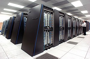
The Blue Gene/P supercomputer at Argonne National Lab runs over 250,000 processors using normal data center air conditioning, grouped in 72 racks/cabinets connected by a high-speed optical network^[1]

A supercomputer is a computer with a high-level computational capacity compared to a general-purpose computer. Performance of a supercomputer is measured in floating point operations per second (FLOPS) instead of million instructions per second (MIPS). As of 2015, there are supercomputers which can perform up to quadrillions of FLOPS.^[2]

Supercomputers were introduced in the 1960s, made initially, and for decades primarily, by Seymour Cray at Control Data Corporation (CDC), Cray Research and subsequent companies bearing his name or monogram. While the supercomputers of the 1970s used only a few processors, in the 1990s machines with thousands of processors began to appear and, by the end of the 20th century, massively parallel supercomputers with tens of thousands of "off-the-shelf" processors were the norm.^[3][4] Since its introduction in June 2013, China's Tianhe-2 supercomputer is currently the fastest in the world at 33.86 petaFLOPS (PFLOPS), or 33.86 quadrillions of FLOPS.

Supercomputers play an important role in the field of computational science, and are used for a wide range of computationally intensive tasks in various fields, including quantum mechanics, weather forecasting, climate research, oil and gas exploration, molecular modeling (computing the structures and properties of chemical compounds, biological macromolecules, polymers, and crystals), and physical simulations (such as simulations of the early moments of the universe, airplane and spacecraft aerodynamics, the detonation of nuclear weapons, and nuclear fusion). Throughout their history, they have been essential in the field of cryptanalysis.^[5]

Systems with massive numbers of processors generally take one of the two paths: in one approach (e.g., in distributed computing), a large number of discrete computers (e.g., laptops) distributed across a network (e.g., the Internet) devote some or all of their time to solving a common problem; each individual computer (client) receives and completes many small tasks, reporting the results to a central server which integrates the task results from all the clients into the overall solution.^[6][7] In another approach, a large number of dedicated processors are placed in close proximity to each other (e.g. in a computer cluster); this saves considerable time moving data around and makes it possible for the processors to work together (rather than on separate tasks), for example in mesh and hypercube architectures.

The use of multi-core processors combined with centralization is an emerging trend; one can think of this as a small cluster (the multicore processor in a smartphone, tablet, laptop, etc.) that both depends upon and contributes to the cloud.^[8][9]

History

A Cray-1 preserved at the Deutsches Museum

The history of supercomputing goes back to the 1960s, with the Atlas at the University of Manchester and a series of computers at Control Data Corporation (CDC), designed by Seymour Cray. These used innovative designs and parallelism to achieve superior computational peak performance.^[10]

The Atlas was a joint venture between Ferranti and the Manchester University and was designed to operate at processing speeds approaching one microsecond per instruction, about one million instructions per second.^[11] The first Atlas was officially commissioned on 7 December 1962 as one of the world's first supercomputers  – considered to be the most powerful computer in the world at that time by a considerable margin, and equivalent to four IBM 7094s.^[12]

The CDC 6600, released in 1964, was designed by Cray to be the fastest in the world. Cray switched from use of germanium to silicon transistors, which could ran very fast, solving the overheating problem by introducing refrigeration.^[13] Given that the 6600 outperformed all the other contemporary computers by about 10 times, it was dubbed a supercomputer and defined the supercomputing market when one hundred computers were sold at $8 million each.^{[14][15][16][17]}

Cray left CDC in 1972 to form his own company, Cray Research.^[15] Four years after leaving CDC, Cray delivered the 80 MHz Cray 1 in 1976, and it became one of the most successful supercomputers in history.^[18][19] The Cray-2 released in 1985 was an 8 processor liquid cooled computer and Fluorinert was pumped through it as it operated. It performed at 1.9 gigaflops and was the world's fastest until 1990.^[20]

While the supercomputers of the 1980s used only a few processors, in the 1990s, machines with thousands of processors began to appear both in the United States and Japan, setting new computational performance records. Fujitsu's Numerical Wind Tunnel supercomputer used 166 vector processors to gain the top spot in 1994 with a peak speed of 1.7 gigaFLOPS (GFLOPS) per processor.^[21][22] The Hitachi SR2201 obtained a peak performance of 600 GFLOPS in 1996 by using 2048 processors connected via a fast three-dimensional crossbar network.^[23][24][25] The Intel Paragon could have 1000 to 4000 Intel i860 processors in various configurations, and was ranked the fastest in the world in 1993. The Paragon was a MIMD machine which connected processors via a high speed two dimensional mesh, allowing processes to execute on separate nodes, communicating via the Message Passing Interface.^[26]

Hardware and architecture

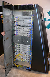
A Blue Gene/L cabinet showing the stacked blades, each holding many processors

Approaches to supercomputer architecture have taken dramatic turns since the earliest systems were introduced in the 1960s. Early supercomputer architectures pioneered by Seymour Cray relied on compact innovative designs and local parallelism to achieve superior computational peak performance.^[10] However, in time the demand for increased computational power ushered in the age of massively parallel systems.

While the supercomputers of the 1970s used only a few processors, in the 1990s, machines with thousands of processors began to appear and by the end of the 20th century, massively parallel supercomputers with tens of thousands of "off-the-shelf" processors were the norm. Supercomputers of the 21st century can use over 100,000 processors (some being graphic units) connected by fast connections.^[3][4] The Connection Machine CM-5 supercomputer is a massively parallel processing computer capable of many billions of arithmetic operations per second.^[27]

Throughout the decades, the management of heat density has remained a key issue for most centralized supercomputers.^[28][29][30] The large amount of heat generated by a system may also have other effects, e.g. reducing the lifetime of other system components.^[31] There have been diverse approaches to heat management, from pumping Fluorinert through the system, to a hybrid liquid-air cooling system or air cooling with normal air conditioning temperatures.^[20][32]

The CPU share of TOP500

Systems with a massive number of processors generally take one of two paths. In the grid computing approach, the processing power of a large number of computers, organised as distributed, diverse administrative domains, is opportunistically used whenever a computer is available.^[6] In another approach, a large number of processors are used in close proximity to each other, e.g. in a computer cluster. In such a centralized massively parallel system the speed and flexibility of the interconnect becomes very important and modern supercomputers have used various approaches ranging from enhanced Infiniband systems to three-dimensional torus interconnects.^[33][34] The use of multi-core processors combined with centralization is an emerging direction, e.g. as in the Cyclops64 system.^[8][9]

As the price, performance and energy efficiency of general purpose graphic processors (GPGPUs) have improved,^[35] a number of petaflop supercomputers such as Tianhe-I and Nebulae have started to rely on them.^[36] However, other systems such as the K computer continue to use conventional processors such as SPARC-based designs and the overall applicability of GPGPUs in general-purpose high-performance computing applications has been the subject of debate, in that while a GPGPU may be tuned to score well on specific benchmarks, its overall applicability to everyday algorithms may be limited unless significant effort is spent to tune the application towards it.^[37][38] However, GPUs are gaining ground and in 2012 the Jaguar supercomputer was transformed into Titan by retrofitting CPUs with GPUs.^[39][40][41]

High performance computers have an expected life cycle of about three years.^[42]

A number of "special-purpose" systems have been designed, dedicated to a single problem. This allows the use of specially programmed FPGA chips or even custom VLSI chips, allowing better price/performance ratios by sacrificing generality. Examples of special-purpose supercomputers include Belle,^[43] Deep Blue,^[44] and Hydra,^[45] for playing chess, Gravity Pipe for astrophysics,^[46] MDGRAPE-3 for protein structure computation molecular dynamics^[47] and Deep Crack,^[48] for breaking the DES cipher.

Energy usage and heat management

A typical supercomputer consumes large amounts of electrical power, almost all of which is converted into heat, requiring cooling. For example, Tianhe-1A consumes 4.04 megawatts of electricity.^[49] The cost to power and cool the system can be significant, e.g. 4 MW at $0.10/kWh is $400 an hour or about $3.5 million per year.

 

An IBM HS20 blade

Heat management is a major issue in complex electronic devices, and affects powerful computer systems in various ways.^[50] The thermal design power and CPU power dissipation issues in supercomputing surpass those of traditional computer cooling technologies. The supercomputing awards for green computing reflect this issue.^[51][52][53]

The packing of thousands of processors together inevitably generates significant amounts of heat density that need to be dealt with. The Cray 2 was liquid cooled, and used a Fluorinert "cooling waterfall" which was forced through the modules under pressure.^[20] However, the submerged liquid cooling approach was not practical for the multi-cabinet systems based on off-the-shelf processors, and in System X a special cooling system that combined air conditioning with liquid cooling was developed in conjunction with the Liebert company.^[32]

In the Blue Gene system, IBM deliberately used low power processors to deal with heat density.^[54] On the other hand, the IBM Power 775, released in 2011, has closely packed elements that require water cooling.^[55] The IBM Aquasar system, on the other hand uses hot water cooling to achieve energy efficiency, the water being used to heat buildings as well.^[56][57]

The energy efficiency of computer systems is generally measured in terms of "FLOPS per watt". In 2008, IBM's Roadrunner operated at 3.76 MFLOPS/W.^[58][59] In November 2010, the Blue Gene/Q reached 1,684 MFLOPS/W.^[60][61] In June 2011 the top 2 spots on the Green 500 list were occupied by Blue Gene machines in New York (one achieving 2097 MFLOPS/W) with the DEGIMA cluster in Nagasaki placing third with 1375 MFLOPS/W.^[62]

Because copper wires can transfer energy into a supercomputer with much higher power densities than forced air or circulating refrigerants can remove waste heat,^[63] the ability of the cooling systems to remove waste heat is a limiting factor.^[64][65] As of 2015^[update], many existing supercomputers have more infrastructure capacity than the actual peak demand of the machine  – designers generally conservatively design the power and cooling infrastructure to handle more than the theoretical peak electrical power consumed by the supercomputer. Designs for future supercomputers are power-limited  – the thermal design power of the supercomputer as a whole, the amount that the power and cooling infrastructure can handle, is somewhat more than the expected normal power consumption, but less than the theoretical peak power consumption of the electronic hardware.^[66]

Software and system management

Operating systems

Since the end of the 20th century, supercomputer operating systems have undergone major transformations, based on the changes in supercomputer architecture.^[67] While early operating systems were custom tailored to each supercomputer to gain speed, the trend has been to move away from in-house operating systems to the adaptation of generic software such as Linux.^[68]
Since modern massively parallel supercomputers typically separate computations from other services by using multiple types of nodes, they usually run different operating systems on different nodes, e.g. using a small and efficient lightweight kernel such as CNK or CNL on compute nodes, but a larger system such as a Linux-derivative on server and I/O nodes.^[69][70][71]

While in a traditional multi-user computer system job scheduling is, in effect, a tasking problem for processing and peripheral resources, in a massively parallel system, the job management system needs to manage the allocation of both computational and communication resources, as well as gracefully deal with inevitable hardware failures when tens of thousands of processors are present.^[72]

Although most modern supercomputers use the Linux operating system, each manufacturer has its own specific Linux-derivative, and no industry standard exists, partly due to the fact that the differences in hardware architectures require changes to optimize the operating system to each hardware design.^[67][73]

Software tools and message passing

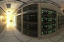
Wide-angle view of the ALMA correlator.^[74]

The parallel architectures of supercomputers often dictate the use of special programming techniques to exploit their speed. Software tools for distributed processing include standard APIs such as MPI and PVM, VTL, and open source-based software solutions such as Beowulf.

In the most common scenario, environments such as PVM and MPI for loosely connected clusters and OpenMP for tightly coordinated shared memory machines are used. Significant effort is required to optimize an algorithm for the interconnect characteristics of the machine it will be run on; the aim is to prevent any of the CPUs from wasting time waiting on data from other nodes. GPGPUs have hundreds of processor cores and are programmed using programming models such as CUDA.

Moreover, it is quite difficult to debug and test parallel programs. Special techniques need to be used for testing and debugging such applications.

Distributed supercomputing

Opportunistic approaches

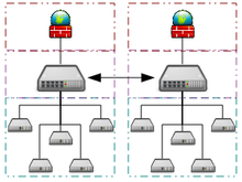
Example architecture of a grid computing system connecting many personal computers over the internet

Opportunistic Supercomputing is a form of networked grid computing whereby a "super virtual computer" of many loosely coupled volunteer computing machines performs very large computing tasks. Grid computing has been applied to a number of large-scale embarrassingly parallel problems that require supercomputing performance scales. However, basic grid and cloud computing approaches that rely on volunteer computing can not handle traditional supercomputing tasks such as fluid dynamic simulations.

The fastest grid computing system is the distributed computing project Folding@home. F@h reported 43.1 PFLOPS of x86 processing power as of June 2014^[update]. Of this, 42.5 PFLOPS are contributed by clients running on various GPUs, and the rest from various CPU systems.^[75]

The BOINC platform hosts a number of distributed computing projects. As of May 2011^[update], BOINC recorded a processing power of over 5.5 PFLOPS through over 480,000 active computers on the network^[76] The most active project (measured by computational power), MilkyWay@home, reports processing power of over 700 teraFLOPS (TFLOPS) through over 33,000 active computers.^[77]

As of May 2011^[update], GIMPS's distributed Mersenne Prime search currently achieves about 60 TFLOPS through over 25,000 registered computers.^[78] The Internet PrimeNet Server supports GIMPS's grid computing approach, one of the earliest and most successful grid computing projects, since 1997.

Quasi-opportunistic approaches

Quasi-opportunistic supercomputing is a form of distributed computing whereby the “super virtual computer” of a large number of networked geographically disperse computers performs computing tasks that demand huge processing power.^[79] Quasi-opportunistic supercomputing aims to provide a higher quality of service than opportunistic grid computing by achieving more control over the assignment of tasks to distributed resources and the use of intelligence about the availability and reliability of individual systems within the supercomputing network. However, quasi-opportunistic distributed execution of demanding parallel computing software in grids should be achieved through implementation of grid-wise allocation agreements, co-allocation subsystems, communication topology-aware allocation mechanisms, fault tolerant message passing libraries and data pre-conditioning.^[79]

Performance measurement

Capability vs capacity

Supercomputers generally aim for the maximum in capability computing rather than capacity computing. Capability computing is typically thought of as using the maximum computing power to solve a single large problem in the shortest amount of time. Often a capability system is able to solve a problem of a size or complexity that no other computer can, e.g. a very complex weather simulation application.^[80]

Capacity computing, in contrast, is typically thought of as using efficient cost-effective computing power to solve a small number of somewhat large problems or a large number of small problems.^[80] Architectures that lend themselves to supporting many users for routine everyday tasks may have a lot of capacity, but are not typically considered supercomputers, given that they do not solve a single very complex problem.^[80]

Performance metrics

Top supercomputer speeds: logscale speed over 60 years

In general, the speed of supercomputers is measured and benchmarked in "FLOPS" (FLoating point Operations Per Second), and not in terms of "MIPS" (Million Instructions Per Second), as is the case with general-purpose computers.^[81] These measurements are commonly used with an SI prefix such as tera-, combined into the shorthand "TFLOPS" (10¹² FLOPS, pronounced teraflops), or peta-, combined into the shorthand "PFLOPS" (10¹⁵ FLOPS, pronounced petaflops.) "Petascale" supercomputers can process one quadrillion (10¹⁵) (1000 trillion) FLOPS. Exascale is computing performance in the exaFLOPS (EFLOPS) range. An EFLOPS is one quintillion (10¹⁸) FLOPS (one million TFLOPS).

No single number can reflect the overall performance of a computer system, yet the goal of the Linpack benchmark is to approximate how fast the computer solves numerical problems and it is widely used in the industry.^[82] The FLOPS measurement is either quoted based on the theoretical floating point performance of a processor (derived from manufacturer's processor specifications and shown as "Rpeak" in the TOP500 lists) which is generally unachievable when running real workloads, or the achievable throughput, derived from the LINPACK benchmarks and shown as "Rmax" in the TOP500 list. The LINPACK benchmark typically performs LU decomposition of a large matrix. The LINPACK performance gives some indication of performance for some real-world problems, but does not necessarily match the processing requirements of many other supercomputer workloads, which for example may require more memory bandwidth, or may require better integer computing performance, or may need a high performance I/O system to achieve high levels of performance.^[82]

The TOP500 list

Distribution of top 500 supercomputers among different countries as of June 2014

Since 1993, the fastest supercomputers have been ranked on the TOP500 list according to their LINPACK benchmark results. The list does not claim to be unbiased or definitive, but it is a widely cited current definition of the "fastest" supercomputer available at any given time.

This is a recent list of the computers which appeared at the top of the TOP500 list,^[83] and the "Peak speed" is given as the "Rmax" rating. For more historical data see History of supercomputing.

Top 20 Supercomputers in the World as of June 2013

Year	Supercomputer	Peak speed (Rmax)	Location
2013	NUDT Tianhe-2	33.86 PFLOPS	Guangzhou, China
2012	Cray Titan	17.59 PFLOPS	Oak Ridge, U.S.
2012	IBM Sequoia	17.17 PFLOPS	Livermore, U.S.
2011	Fujitsu K computer	10.51 PFLOPS	Kobe, Japan
2010	Tianhe-IA	2.566 PFLOPS	Tianjin, China
2009	Cray Jaguar	1.759 PFLOPS	Oak Ridge, U.S.
2008	IBM Roadrunner	1.026 PFLOPS	Los Alamos, U.S.
		1.105 PFLOPS

Largest Supercomputer Vendors according to the total Rmax (GFLOPS) operated

Source : TOP500

Country/Vendor	System count	System share (%)	Rmax (GFLOPS)	Rpeak (GFLOPS)	Processor cores
IBM	153	30.6	87,143,814	122,311,749	7,346,514
Cray Inc.	62	12.4	68,198,477	97,027,365	3,583,180
HP	179	35.8	44,855,405	73,630,508	3,747,812
NUDT	5	1	39,483,490	64,356,373	3,547,648
SGI	23	4.6	14,741,773	17,963,102	813,376
Fujitsu	8	1.6	13,719,473	14,981,840	915,974
Bull	18	3.6	10,094,490	12,564,851	588,120
Dell	9	1.8	8,003,573	12,687,479	618,396
Atipa	3	0.6	3,044,976	4,163,712	214,584
NEC/HP	1	0.2	2,785,000	5,735,685	76,032
T-Platforms	2	0.4	2,750,900	4,276,082	115,780
RSC Group	4	0.8	1,492,512	2,399,433	99,200
Dawning	2	0.4	1,451,600	3,217,772	151,360
Hitachi/Fujitsu	1	0.2	1,018,000	1,502,236	222,072
Supermicro	1	0.2	798,261	3,164,480	160,600
NRCPCET	1	0.2	795,900	1,070,160	137,200
ClusterVision	2	0.4	784,735	881,254	42,368
Intel	1	0.2	758,873	933,481	51,392
Amazon	2	0.4	724,269	947,610	43,520
Oracle	2	0.4	708,300	804,835	68,672
MEGWARE	3	0.6	610,521	710,592	54,800
NEC	3	0.6	578,987	709,520	21,296
Adtech	1	0.2	532,600	1,098,000	38,400
Hitachi	2	0.4	496,900	622,598	20,544
IPE, Nvidia, Tyan	1	0.2	496,500	1,012,650	29,440
Itautec	2	0.4	411,800	920,830	27,776
Netweb Technologies	1	0.2	388,442	520,358	30,056
Xenon Systems	1	0.2	335,300	472,498	6,875
AMD, ASUS, FIAS, GSI	1	0.2	316,700	593,600	10,976
Clustervision/Supermicro	1	0.2	299,300	588,749	44,928
Niagara Computers, Supermicro	1	0.2	289,500	348,660	5,310
Inspur	1	0.2	196,234	262,560	8,412
HP/WIPRO	1	0.2	188,700	394,760	12,532
PEZY Computing/Exascaler Inc.	1	0.2	178,107	395,264	262,784
Acer Group	1	0.2	177,100	231,859	26,244

Applications

The stages of supercomputer application may be summarized in the following table:

Decade	Uses and computer involved
1970s	Weather forecasting, aerodynamic research (Cray-1).[84]
1980s	Probabilistic analysis,[85] radiation shielding modeling[86] (CDC Cyber).
1990s	Brute force code breaking (EFF DES cracker).[87]
2000s	3D nuclear test simulations as a substitute for legal conduct Nuclear Non-Proliferation Treaty (ASCI Q).[88]
2010s	Molecular Dynamics Simulation (Tianhe-1A)[89]

The IBM Blue Gene/P computer has been used to simulate a number of artificial neurons equivalent to approximately one percent of a human cerebral cortex, containing 1.6 billion neurons with approximately 9 trillion connections. The same research group also succeeded in using a supercomputer to simulate a number of artificial neurons equivalent to the entirety of a rat's brain.^[90]

Modern-day weather forecasting also relies on supercomputers. The National Oceanic and Atmospheric Administration uses supercomputers to crunch hundreds of millions of observations to help make weather forecasts more accurate.^[91]

In 2011, the challenges and difficulties in pushing the envelope in supercomputing were underscored by IBM's abandonment of the Blue Waters petascale project.^[92]

Research and development trends

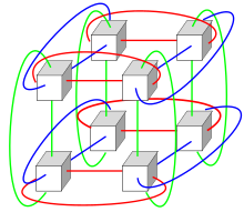
Diagram of a 3-dimensional torus interconnect used by systems such as Blue Gene, Cray XT3, etc.

Given the current speed of progress, industry experts estimate that supercomputers will reach 1 EFLOPS (10¹⁸, 1,000 PFLOPS or one quintillion FLOPS) by 2018. The Chinese government in particular is pushing to achieve this goal after they briefly achieved the most powerful supercomputer in the world with Tianhe-1A in 2010 (ranked fifth by 2012).^[93] Using the Intel MIC multi-core processor architecture, which is Intel's response to GPU systems, SGI also plans to achieve a 500-fold increase in performance by 2018 in order to achieve one EFLOPS. Samples of MIC chips with 32 cores, which combine vector processing units with standard CPU, have become available.^[94] The Indian government has also stated ambitions for an EFLOPS-range supercomputer, which they hope to complete by 2017.^[95] In November 2014, it was reported that India is working on the fastest supercomputer ever, which is set to work at 132 EFLOPS.^[96]

Erik P. DeBenedictis of Sandia National Laboratories theorizes that a zettaFLOPS (10²¹, one sextillion FLOPS) computer is required to accomplish full weather modeling, which could cover a two-week time span accurately.^{[97][not in citation given]} Such systems might be built around 2030.^[98]

Energy use

High performance supercomputers usually require high energy, as well. However, Iceland may be a benchmark for the future with the world's first zero-emission supercomputer. Located at the Thor Data Center in Reykjavik, Iceland, this supercomputer relies on completely renewable sources for its power rather than fossil fuels. The colder climate is an added bonus for help with cooling, too, making it one of the greenest facilities in the world. ^[99]