Coherence (physics)

From Wikipedia, the free encyclopedia

https://en.wikipedia.org/wiki/Coherence_(physics)

In physics, coherence expresses the potential for two waves to interfere. Two monochromatic beams from a single source always interfere. Physical sources are not strictly monochromatic: they may be partly coherent. Beams from different sources are mutually incoherent.

When interfering, two waves add together to create a wave of greater amplitude than either one (constructive interference) or subtract from each other to create a wave of minima which may be zero (destructive interference), depending on their relative phase. Constructive or destructive interference are limit cases, and two waves always interfere, even if the result of the addition is complicated or not remarkable.

Two waves with constant relative phase will be coherent. The amount of coherence can readily be measured by the interference visibility, which looks at the size of the interference fringes relative to the input waves (as the phase offset is varied); a precise mathematical definition of the degree of coherence is given by means of correlation functions. More generally, coherence describes the statistical similarity of a field (electromagnetic field, quantum wave packet etc.) at two points in space or time.

Qualitative concept

Two slits illuminated by one source show an interference pattern. The source is far to the left in the diagram, behind collimators that create a parallel beam. This combination ensures that a wave from the source strikes both slits at the same part of the wave cycle: the wave will have coherence.

Coherence controls the visibility or contrast of interference patterns. For example, visibility of the double slit experiment pattern requires that both slits be illuminated by a coherent wave as illustrated in the figure. Large sources without collimation or sources that mix many different frequencies will have lower visibility.

Coherence contains several distinct concepts. Spatial coherence describes the correlation (or predictable relationship) between waves at different points in space, either lateral or longitudinal. Temporal coherence describes the correlation between waves observed at different moments in time. Both are observed in the Michelson–Morley experiment and Young's interference experiment. Once the fringes are obtained in the Michelson interferometer, when one of the mirrors is moved away gradually from the beam-splitter, the time for the beam to travel increases and the fringes become dull and finally disappear, showing temporal coherence. Similarly, in a double-slit experiment, if the space between the two slits is increased, the coherence dies gradually and finally the fringes disappear, showing spatial coherence. In both cases, the fringe amplitude slowly disappears, as the path difference increases past the coherence length.

Coherence was originally conceived in connection with Thomas Young's double-slit experiment in optics but is now used in any field that involves waves, such as acoustics, electrical engineering, neuroscience, and quantum mechanics. The property of coherence is the basis for commercial applications such as holography, the Sagnac gyroscope, radio antenna arrays, optical coherence tomography and telescope interferometers (Astronomical optical interferometers and radio telescopes).

Mathematical definition

Further information: Degree of coherence

The coherence function between two signals ${\displaystyle x(t)}$ and ${\displaystyle y(t)}$ is defined as

${\displaystyle {\gamma }_{xy}^2(f)=\frac{|S_{xy}(f){|}^2}{S_{xx}(f)S_{yy}(f)}}$

where ${\displaystyle S_{xy}(f)}$ is the cross-spectral density of the signal and ${\displaystyle S_{xx}(f)}$ and ${\displaystyle S_{yy}(f)}$ are the power spectral density functions of ${\displaystyle x(t)}$ and ${\displaystyle y(t)}$, respectively. The cross-spectral density and the power spectral density are defined as the Fourier transforms of the cross-correlation and the autocorrelation signals, respectively. For instance, if the signals are functions of time, the cross-correlation is a measure of the similarity of the two signals as a function of the time lag relative to each other and the autocorrelation is a measure of the similarity of each signal with itself in different instants of time. In this case the coherence is a function of frequency. Analogously, if ${\displaystyle x(t)}$ and ${\displaystyle y(t)}$ are functions of space, the cross-correlation measures the similarity of two signals in different points in space and the autocorrelations the similarity of the signal relative to itself for a certain separation distance. In that case, coherence is a function of wavenumber (spatial frequency).

The coherence varies in the interval ${\displaystyle 0\le {\gamma }_{xy}^2(f)\le 1}$. If ${\displaystyle {\gamma }_{xy}^2(f)=1}$ it means that the signals are perfectly correlated or linearly related and if ${\displaystyle {\gamma }_{xy}^2(f)=0}$ they are totally uncorrelated. If a linear system is being measured, ${\displaystyle x(t)}$ being the input and ${\displaystyle y(t)}$ the output, the coherence function will be unitary all over the spectrum. However, if non-linearities are present in the system the coherence will vary in the limit given above.

Coherence and correlation

The coherence of two waves expresses how well correlated the waves are as quantified by the cross-correlation function. Cross-correlation quantifies the ability to predict the phase of the second wave by knowing the phase of the first. As an example, consider two waves perfectly correlated for all times (by using a monochromatic light source). At any time, the phase difference between the two waves will be constant. If, when they are combined, they exhibit perfect constructive interference, perfect destructive interference, or something in-between but with constant phase difference, then it follows that they are perfectly coherent. As will be discussed below, the second wave need not be a separate entity. It could be the first wave at a different time or position. In this case, the measure of correlation is the autocorrelation function (sometimes called self-coherence). Degree of correlation involves correlation functions.

Examples of wave-like states

These states are unified by the fact that their behavior is described by a wave equation or some generalization thereof.

• Waves in a rope (up and down) or slinky (compression and expansion)
• Surface waves in a liquid
• Electromagnetic signals (fields) in transmission lines
• Sound
• Radio waves and microwaves
• Light waves (optics)
• Matter waves associated with, for examples, electrons and atoms

In system with macroscopic waves, one can measure the wave directly. Consequently, its correlation with another wave can simply be calculated. However, in optics one cannot measure the electric field directly as it oscillates much faster than any detector's time resolution. Instead, one measures the intensity of the light. Most of the concepts involving coherence which will be introduced below were developed in the field of optics and then used in other fields. Therefore, many of the standard measurements of coherence are indirect measurements, even in fields where the wave can be measured directly.

Temporal coherence

Figure 1: The amplitude of a single frequency wave as a function of time t (red) and a copy of the same wave delayed by ${\displaystyle \tau }$ (blue). The coherence time of the wave is infinite since it is perfectly correlated with itself for all delays ${\displaystyle \tau }$.

Figure 2: The amplitude of a wave whose phase drifts significantly in time ${\displaystyle {\tau }_{\mathrm{c}}}$ as a function of time t (red) and a copy of the same wave delayed by ${\displaystyle 2\tau }$(green). At any particular time t the wave can interfere perfectly with its delayed copy. But, since half the time the red and green waves are in phase and half the time out of phase, when averaged over t any interference disappears at this delay.

Temporal coherence is the measure of the average correlation between the value of a wave and itself delayed by ${\displaystyle \tau }$, at any pair of times. Temporal coherence tells us how monochromatic a source is. In other words, it characterizes how well a wave can interfere with itself at a different time. The delay over which the phase or amplitude wanders by a significant amount (and hence the correlation decreases by significant amount) is defined as the coherence time ${\displaystyle {\tau }_{\mathrm{c}}}$. At a delay of ${\displaystyle \tau =0}$ the degree of coherence is perfect, whereas it drops significantly as the delay passes ${\displaystyle \tau ={\tau }_{\mathrm{c}}}$. The coherence length ${\displaystyle L_{\mathrm{c}}}$ is defined as the distance the wave travels in time ${\displaystyle {\tau }_{\mathrm{c}}}$.

The coherence time is not the time duration of the signal; the coherence length differs from the coherence area (see below).

The relationship between coherence time and bandwidth

The larger the bandwidth – range of frequencies Δf a wave contains – the faster the wave decorrelates (and hence the smaller ${\displaystyle {\tau }_{\mathrm{c}}}$ is)

${\displaystyle {\tau }_c\mathrm{\Delta }f\gtrsim 1.}$

Formally, this follows from the convolution theorem in mathematics, which relates the Fourier transform of the power spectrum (the intensity of each frequency) to its autocorrelation.

Narrow bandwidth lasers have long coherence lengths (up to hundreds of meters). For example, a stabilized and monomode helium–neon laser can easily produce light with coherence lengths of 300 m. Not all lasers have a highly monochromaticity, however (e.g. for a mode-locked Ti-sapphire laser, Δλ ≈ 2 nm – 70 nm).

LEDs are characterized by Δλ ≈ 50 nm, and tungsten filament lights exhibit Δλ ≈ 600 nm, so these sources have shorter coherence times than the most monochromatic lasers.

Examples of temporal coherence

Examples of temporal coherence include:

• A wave containing only a single frequency (monochromatic) is perfectly correlated with itself at all time delays, in accordance with the above relation. (See Figure 1)
• Conversely, a wave whose phase drifts quickly will have a short coherence time. (See Figure 2)
• Similarly, pulses (wave packets) of waves, which naturally have a broad range of frequencies, also have a short coherence time since the amplitude of the wave changes quickly. (See Figure 3)
• Finally, white light, which has a very broad range of frequencies, is a wave which varies quickly in both amplitude and phase. Since it consequently has a very short coherence time (just 10 periods or so), it is often called incoherent.

Holography requires light with a long coherence time. In contrast, optical coherence tomography, in its classical version, uses light with a short coherence time.

Measurement of temporal coherence

Figure 3: The amplitude of a wavepacket whose amplitude changes significantly in time ${\displaystyle {\tau }_{\mathrm{c}}}$ (red) and a copy of the same wave delayed by ${\displaystyle 2\tau }$(green) plotted as a function of time t. At any particular time the red and green waves are uncorrelated; one oscillates while the other is constant and so there will be no interference at this delay. Another way of looking at this is the wavepackets are not overlapped in time and so at any particular time there is only one nonzero field so no interference can occur.

Figure 4: The time-averaged intensity (blue) detected at the output of an interferometer plotted as a function of delay τ for the example waves in Figures 2 and 3. As the delay is changed by half a period, the interference switches between constructive and destructive. The black lines indicate the interference envelope, which gives the degree of coherence. Although the waves in Figures 2 and 3 have different time durations, they have the same coherence time.

In optics, temporal coherence is measured in an interferometer such as the Michelson interferometer or Mach–Zehnder interferometer. In these devices, a wave is combined with a copy of itself that is delayed by time ${\displaystyle \tau }$. A detector measures the time-averaged intensity of the light exiting the interferometer. The resulting visibility of the interference pattern (e.g. see Figure 4) gives the temporal coherence at delay ${\displaystyle \tau }$. Since for most natural light sources, the coherence time is much shorter than the time resolution of any detector, the detector itself does the time averaging. Consider the example shown in Figure 3. At a fixed delay, here ${\displaystyle 2\tau }$, an infinitely fast detector would measure an intensity that fluctuates significantly over a time t equal to ${\displaystyle \tau }$. In this case, to find the temporal coherence at ${\displaystyle 2{\tau }_{\mathrm{c}}}$, one would manually time-average the intensity.

Spatial coherence

In some systems, such as water waves or optics, wave-like states can extend over one or two dimensions. Spatial coherence describes the ability for two spatial points x₁ and x₂ in the extent of a wave to interfere when averaged over time. More precisely, the spatial coherence is the cross-correlation between two points in a wave for all times. If a wave has only 1 value of amplitude over an infinite length, it is perfectly spatially coherent. The range of separation between the two points over which there is significant interference defines the diameter of the coherence area, ${\displaystyle A_{\mathrm{c}}}$, (Coherence length ${\displaystyle l_{\mathrm{c}}}$, often a feature of a source, is usually an industrial term related to the coherence time of the source, not the coherence area in the medium.) ${\displaystyle A_{\mathrm{c}}}$ is the relevant type of coherence for the Young's double-slit interferometer. It is also used in optical imaging systems and particularly in various types of astronomy telescopes. Sometimes people also use "spatial coherence" to refer to the visibility when a wave-like state is combined with a spatially shifted copy of itself.

Examples

• Spatial coherence
• 
  Figure 5: A plane wave with an infinite coherence length.
• 
  Figure 6: A wave with a varying profile (wavefront) and infinite coherence length.
• 
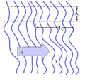  Figure 7: A wave with a varying profile (wavefront) and finite coherence length.
• 
  Figure 8: A wave with finite coherence area is incident on a pinhole (small aperture). The wave will diffract out of the pinhole. Far from the pinhole the emerging spherical wavefronts are approximately flat. The coherence area is now infinite while the coherence length is unchanged.
• 
  Figure 9: A wave with infinite coherence area is combined with a spatially shifted copy of itself. Some sections in the wave interfere constructively and some will interfere destructively. Averaging over these sections, a detector with length D will measure reduced interference visibility. For example, a misaligned Mach–Zehnder interferometer will do this.

Consider a tungsten light-bulb filament. Different points in the filament emit light independently and have no fixed phase-relationship. In detail, at any point in time the profile of the emitted light is going to be distorted. The profile will change randomly over the coherence time ${\displaystyle {\tau }_c}$. Since for a white-light source such as a light-bulb ${\displaystyle {\tau }_c}$ is small, the filament is considered a spatially incoherent source. In contrast, a radio antenna array, has large spatial coherence because antennas at opposite ends of the array emit with a fixed phase-relationship. Light waves produced by a laser often have high temporal and spatial coherence (though the degree of coherence depends strongly on the exact properties of the laser). Spatial coherence of laser beams also manifests itself as speckle patterns and diffraction fringes seen at the edges of shadow.

Holography requires temporally and spatially coherent light. Its inventor, Dennis Gabor, produced successful holograms more than ten years before lasers were invented. To produce coherent light he passed the monochromatic light from an emission line of a mercury-vapor lamp through a pinhole spatial filter.

In February 2011 it was reported that helium atoms, cooled to near absolute zero / Bose–Einstein condensate state, can be made to flow and behave as a coherent beam as occurs in a laser. Moreover, the coherence properties of the output light from multimode nonlinear optical structures were found to obey the optical thermodynamic theory.

Spectral coherence of short pulses

Figure 10: Waves of different frequencies interfere to form a localized pulse if they are coherent.

Figure 11: Spectrally incoherent light interferes to form continuous light with a randomly varying phase and amplitude

Waves of different frequencies (in light these are different colours) can interfere to form a pulse if they have a fixed relative phase-relationship (see Fourier transform). Conversely, if waves of different frequencies are not coherent, then, when combined, they create a wave that is continuous in time (e.g. white light or white noise). The temporal duration of the pulse ${\displaystyle \mathrm{\Delta }t}$ is limited by the spectral bandwidth of the light ${\displaystyle \mathrm{\Delta }f}$ according to:

${\displaystyle \mathrm{\Delta }f\mathrm{\Delta }t\ge 1}$,

which follows from the properties of the Fourier transform and results in Küpfmüller's uncertainty principle (for quantum particles it also results in the Heisenberg uncertainty principle).

If the phase depends linearly on the frequency (i.e. ${\displaystyle \theta (f)\propto f}$) then the pulse will have the minimum time duration for its bandwidth (a transform-limited pulse), otherwise it is chirped (see dispersion).

Measurement of spectral coherence

Measurement of the spectral coherence of light requires a nonlinear optical interferometer, such as an intensity optical correlator, frequency-resolved optical gating (FROG), or spectral phase interferometry for direct electric-field reconstruction (SPIDER).

Polarization and coherence

Further information: Unpolarized light

Light also has a polarization, which is the direction in which the electric or magnetic field oscillates. Unpolarized light is composed of incoherent light waves with random polarization angles. The electric field of the unpolarized light wanders in every direction and changes in phase over the coherence time of the two light waves. An absorbing polarizer rotated to any angle will always transmit half the incident intensity when averaged over time.

If the electric field wanders by a smaller amount the light will be partially polarized so that at some angle, the polarizer will transmit more than half the intensity. If a wave is combined with an orthogonally polarized copy of itself delayed by less than the coherence time, partially polarized light is created.

The polarization of a light beam is represented by a vector in the Poincaré sphere. For polarized light the end of the vector lies on the surface of the sphere, whereas the vector has zero length for unpolarized light. The vector for partially polarized light lies within the sphere.

Quantum coherence

Further information: Quantum decoherence

The signature property of quantum matter waves, wave interference, relies on coherence. While initially patterned after optical coherence, the theory and experimental understanding of quantum coherence greatly expanded the topic.

Matter wave coherence

The simplest extension of optical coherence applies optical concepts to matter waves. For example, when performing the double-slit experiment with atoms in place of light waves, a sufficiently collimated atomic beam creates a coherent atomic wave-function illuminating both slits. Each slit acts as a separate but in-phase beam contributing to the intensity pattern on a screen. These two contributions give rise to an intensity pattern of bright bands due to constructive interference, interlaced with dark bands due to destructive interference, on a downstream screen. Many variations of this experiment have been demonstrated.

As with light, transverse coherence (across the direction of propagation) of matter waves is controlled by collimation. Because light, at all frequencies, travels the same velocity, longitudinal and temporal coherence are linked; in matter waves these are independent. In matter waves, velocity (energy) selection controls longitudinal coherence and pulsing or chopping controls temporal coherence.

Quantum optics

The discovery of the Hanbury Brown and Twiss effect – correlation of light upon coincidence – triggered Glauber's creation of uniquely quantum coherence analysis. Classical optical coherence becomes a classical limit for first-order quantum coherence; higher degree of coherence leads to many phenomena in quantum optics.

Macroscopic quantum coherence

Macroscopic scale quantum coherence leads to novel phenomena, the so-called macroscopic quantum phenomena. For instance, the laser, superconductivity and superfluidity are examples of highly coherent quantum systems whose effects are evident at the macroscopic scale. The macroscopic quantum coherence (off-diagonal long-range order, ODLRO) for superfluidity, and laser light, is related to first-order (1-body) coherence/ODLRO, while superconductivity is related to second-order coherence/ODLRO. (For fermions, such as electrons, only even orders of coherence/ODLRO are possible.) For bosons, a Bose–Einstein condensate is an example of a system exhibiting macroscopic quantum coherence through a multiple occupied single-particle state.

The classical electromagnetic field exhibits macroscopic quantum coherence. The most obvious example is the carrier signal for radio and TV. They satisfy Glauber's quantum description of coherence.

Quantum coherence as a resource

Recently M. B. Plenio and co-workers constructed an operational formulation of quantum coherence as a resource theory. They introduced coherence monotones analogous to the entanglement monotones. Quantum coherence has been shown to be equivalent to quantum entanglement in the sense that coherence can be faithfully described as entanglement, and conversely that each entanglement measure corresponds to a coherence measure.

Applications

Holography

Coherent superpositions of optical wave fields include holography. Holographic photographs have been used as art and as difficult to forge security labels.

Non-optical wave fields

Further applications concern the coherent superposition of non-optical wave fields. In quantum mechanics for example one considers a probability field, which is related to the wave function ${\displaystyle \psi (\mathbf{r})}$ (interpretation: density of the probability amplitude). Here the applications concern, among others, the future technologies of quantum computing and the already available technology of quantum cryptography. Additionally the problems of the following subchapter are treated.

Modal analysis

Coherence is used to check the quality of the transfer functions (FRFs) being measured. Low coherence can be caused by poor signal to noise ratio, and/or inadequate frequency resolution.

Degrees of freedom (mechanics)

From Wikipedia, the free encyclopedia

https://en.wikipedia.org/wiki/Degrees_of_freedom_(mechanics)

In physics, the degrees of freedom (DOF) of a mechanical system is the number of independent parameters that define its configuration or state. It is important in the analysis of systems of bodies in mechanical engineering, structural engineering, aerospace engineering, robotics, and other fields.

The position of a single railcar (engine) moving along a track has one degree of freedom because the position of the car is defined by the distance along the track. A train of rigid cars connected by hinges to an engine still has only one degree of freedom because the positions of the cars behind the engine are constrained by the shape of the track.

An automobile with highly stiff suspension can be considered to be a rigid body traveling on a plane (a flat, two-dimensional space). This body has three independent degrees of freedom consisting of two components of translation and one angle of rotation. Skidding or drifting is a good example of an automobile's three independent degrees of freedom.

The position and orientation of a rigid body in space is defined by three components of translation and three components of rotation, which means that it has six degrees of freedom.

The exact constraint mechanical design method manages the degrees of freedom to neither underconstrain nor overconstrain a device.

Motions and dimensions

The position of an n-dimensional rigid body is defined by the rigid transformation, [T] = [A, d], where d is an n-dimensional translation and A is an n × n rotation matrix, which has n translational degrees of freedom and n(n − 1)/2 rotational degrees of freedom. The number of rotational degrees of freedom comes from the dimension of the rotation group SO(n).

A non-rigid or deformable body may be thought of as a collection of many minute particles (infinite number of DOFs), this is often approximated by a finite DOF system. When motion involving large displacements is the main objective of study (e.g. for analyzing the motion of satellites), a deformable body may be approximated as a rigid body (or even a particle) in order to simplify the analysis.

The degree of freedom of a system can be viewed as the minimum number of coordinates required to specify a configuration. Applying this definition, we have:

1. For a single particle in a plane two coordinates define its location so it has two degrees of freedom;
2. A single particle in space requires three coordinates so it has three degrees of freedom;
3. Two particles in space have a combined six degrees of freedom;
4. If two particles in space are constrained to maintain a constant distance from each other, such as in the case of a diatomic molecule, then the six coordinates must satisfy a single constraint equation defined by the distance formula. This reduces the degree of freedom of the system to five, because the distance formula can be used to solve for the remaining coordinate once the other five are specified.

Rigid bodies

The six degrees of freedom of movement of a ship

Altitude degrees of freedom for an airplane

Mnemonics to remember angle names

Main article: Six degrees of freedom

A single rigid body has at most six degrees of freedom (6 DOF) 3T3R consisting of three translations 3T and three rotations 3R.

See also Euler angles.

For example, the motion of a ship at sea has the six degrees of freedom of a rigid body, and is described as:

Translation and rotation:

1. Walking (or surging): Moving forward and backward;
2. Strafing (or swaying): Moving left and right;
3. Elevating (or heaving): Moving up and down;
4. Roll rotation: Pivots side to side;
5. Pitch rotation: Tilts forward and backward;
6. Yaw rotation: Swivels left and right;

For example, the trajectory of an airplane in flight has three degrees of freedom and its attitude along the trajectory has three degrees of freedom, for a total of six degrees of freedom.

• For rolling in flight and ship dynamics, see roll (aviation) and roll (ship motion), respectively.
  • An important derivative is the roll rate (or roll velocity), which is the angular speed at which an aircraft can change its roll attitude, and is typically expressed in degrees per second.
• For pitching in flight and ship dynamics, see pitch (aviation) and pitch (ship motion), respectively.
• For yawing in flight and ship dynamics, see yaw (aviation) and yaw (ship motion), respectively.
  • One important derivative is the yaw rate (or yaw velocity), the angular speed of yaw rotation, measured with a yaw rate sensor.
  • Another important derivative is the yawing moment, the angular momentum of a yaw rotation, which is important for adverse yaw in aircraft dynamics.

Lower mobility

See also: Parallel manipulator

Physical constraints may limit the number of degrees of freedom of a single rigid body.  For example, a block sliding around on a flat table has 3 DOF 2T1R consisting of two translations 2T and 1 rotation 1R.  An XYZ positioning robot like SCARA has 3 DOF 3T lower mobility.

Mobility formula

The mobility formula counts the number of parameters that define the configuration of a set of rigid bodies that are constrained by joints connecting these bodies.

Consider a system of n rigid bodies moving in space has 6n degrees of freedom measured relative to a fixed frame. In order to count the degrees of freedom of this system, include the fixed body in the count of bodies, so that mobility is independent of the choice of the body that forms the fixed frame. Then the degree-of-freedom of the unconstrained system of N = n + 1 is

${\displaystyle M=6n=6(N-1),}$

because the fixed body has zero degrees of freedom relative to itself.

Joints that connect bodies in this system remove degrees of freedom and reduce mobility. Specifically, hinges and sliders each impose five constraints and therefore remove five degrees of freedom. It is convenient to define the number of constraints c that a joint imposes in terms of the joint's freedom f, where c = 6 − f. In the case of a hinge or slider, which are one degree of freedom joints, have f = 1 and therefore c = 6 − 1 = 5.

The result is that the mobility of a system formed from n moving links and j joints each with freedom f_i, i = 1, ..., j, is given by

${\displaystyle M=6n-\sum _{i=1}^j(6-f_i)=6(N-1-j)+\sum _{i=1}^j{f}_i}$

Recall that N includes the fixed link.

There are two important special cases: (i) a simple open chain, and (ii) a simple closed chain. A single open chain consists of n moving links connected end to end by n joints, with one end connected to a ground link. Thus, in this case N = j + 1 and the mobility of the chain is

${\displaystyle M=\sum _{i=1}^j{f}_i}$

For a simple closed chain, n moving links are connected end-to-end by n + 1 joints such that the two ends are connected to the ground link forming a loop. In this case, we have N = j and the mobility of the chain is

${\displaystyle M=\sum _{i=1}^j{f}_i-6}$

An example of a simple open chain is a serial robot manipulator. These robotic systems are constructed from a series of links connected by six one degree-of-freedom revolute or prismatic joints, so the system has six degrees of freedom.

An example of a simple closed chain is the RSSR spatial four-bar linkage. The sum of the freedom of these joints is eight, so the mobility of the linkage is two, where one of the degrees of freedom is the rotation of the coupler around the line joining the two S joints.

Planar and spherical movement

It is common practice to design the linkage system so that the movement of all of the bodies are constrained to lie on parallel planes, to form what is known as a planar linkage. It is also possible to construct the linkage system so that all of the bodies move on concentric spheres, forming a spherical linkage. In both cases, the degrees of freedom of the links in each system is now three rather than six, and the constraints imposed by joints are now c = 3 − f.

In this case, the mobility formula is given by

${\displaystyle M=3(N-1-j)+\sum _{i=1}^j{f}_i,}$

and the special cases become

• planar or spherical simple open chain,
  $${\displaystyle M=\sum _{i=1}^j{f}_i,}$$

  
• planar or spherical simple closed chain,
  $${\displaystyle M=\sum _{i=1}^j{f}_i-3.}$$

  

An example of a planar simple closed chain is the planar four-bar linkage, which is a four-bar loop with four one degree-of-freedom joints and therefore has mobility M = 1.

Systems of bodies

An articulated robot with six DOF in a kinematic chain.

A system with several bodies would have a combined DOF that is the sum of the DOFs of the bodies, less the internal constraints they may have on relative motion. A mechanism or linkage containing a number of connected rigid bodies may have more than the degrees of freedom for a single rigid body. Here the term degrees of freedom is used to describe the number of parameters needed to specify the spatial pose of a linkage. It is also defined in context of the configuration space, task space and workspace of a robot.

A specific type of linkage is the open kinematic chain, where a set of rigid links are connected at joints; a joint may provide one DOF (hinge/sliding), or two (cylindrical). Such chains occur commonly in robotics, biomechanics, and for satellites and other space structures. A human arm is considered to have seven DOFs. A shoulder gives pitch,yaw, and roll, an elbow allows for pitch, and a wrist allows for pitch, yaw and roll. Only 3 of those movements would be necessary to move the hand to any point in space, but people would lack the ability to grasp things from different angles or directions. A robot (or object) that has mechanisms to control all 6 physical DOF is said to be holonomic. An object with fewer controllable DOFs than total DOFs is said to be non-holonomic, and an object with more controllable DOFs than total DOFs (such as the human arm) is said to be redundant. Although keep in mind that it is not redundant in the human arm because the two DOFs; wrist and shoulder, that represent the same movement; roll, supply each other since they can't do a full 360. The degree of freedom are like different movements that can be made.

In mobile robotics, a car-like robot can reach any position and orientation in 2-D space, so it needs 3 DOFs to describe its pose, but at any point, you can move it only by a forward motion and a steering angle. So it has two control DOFs and three representational DOFs; i.e. it is non-holonomic. A fixed-wing aircraft, with 3–4 control DOFs (forward motion, roll, pitch, and to a limited extent, yaw) in a 3-D space, is also non-holonomic, as it cannot move directly up/down or left/right.

A summary of formulas and methods for computing the degrees-of-freedom in mechanical systems has been given by Pennestri, Cavacece, and Vita.

Electrical engineering

In electrical engineering degrees of freedom is often used to describe the number of directions in which a phased array antenna can form either beams or nulls. It is equal to one less than the number of elements contained in the array, as one element is used as a reference against which either constructive or destructive interference may be applied using each of the remaining antenna elements. Radar practice and communication link practice, with beam steering being more prevalent for radar applications and null steering being more prevalent for interference suppression in communication links.