Life on Venus

From Wikipedia, the free encyclopedia

https://en.wikipedia.org/wiki/Life_on_Venus 

The atmosphere of Venus as viewed in ultraviolet by the Pioneer Venus Orbiter in 1979. The cause of the dark streaks in the clouds is not yet known.

The possibility of life on Venus is a subject of interest in astrobiology due to Venus's proximity and similarities to Earth. To date, no definitive evidence has been found of past or present life there. In the early 1960s, studies conducted via spacecraft demonstrated that the current Venusian environment is extreme compared to Earth's. Studies continue to question whether life could have existed on the planet's surface before a runaway greenhouse effect took hold, and whether a relict biosphere could persist high in the modern Venusian atmosphere.

With extreme surface temperatures reaching nearly 735 K (462 °C; 863 °F) and an atmospheric pressure 92 times that of Earth, the conditions on Venus make water-based life as we know it unlikely on the surface of the planet. However, a few scientists have speculated that thermoacidophilic extremophile microorganisms might exist in the temperate, acidic upper layers of the Venusian atmosphere. In September 2020, research was published that reported the presence of phosphine in the planet's atmosphere, a potential biosignature. However, doubts have been cast on these observations.

As of 8 February 2021, an updated status of studies considering the possible detection of lifeforms on Venus (via phosphine) and Mars (via methane) was reported, though whether these gases are present is still unclear. On 2 June 2021, NASA announced two new related missions to Venus: DAVINCI and VERITAS.

Surface conditions

Main article: Observations and explorations of Venus

Venus as photographed by Mariner 10

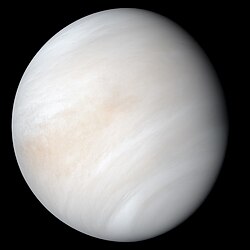
Because Venus is completely covered in clouds, human knowledge of surface conditions was largely speculative until the space probe era. Until the mid-20th century, the surface environment of Venus was believed to be similar to Earth, hence it was widely believed that Venus could harbor life. In 1870, the British astronomer Richard A. Proctor said the existence of life on Venus was impossible near its equator, but possible near its poles.

Microwave observations published by C. Mayer et al. in 1958 indicated a high-temperature source (600 K). Strangely, millimetre-band observations made by A. D. Kuzmin indicated much lower temperatures. Two competing theories explained the unusual radio spectrum, one suggesting the high temperatures originated in the ionosphere, and another suggesting a hot planetary surface.

In 1962, Mariner 2, the first successful mission to Venus, measured the planet's temperature for the first time, and found it to be "about 500 degrees Celsius (900 degrees Fahrenheit)." Since then, increasingly clear evidence from various space probes showed Venus has an extreme climate, with a greenhouse effect generating a constant temperature of about 500 °C (932 °F) on the surface. The atmosphere contains sulfuric acid clouds. In 1968, NASA reported that air pressure on the Venusian surface was 75 to 100 times that of Earth. This was later revised to 92 bars, almost 100 times that of Earth and similar to that of more than 1,000 m (3,300 ft) deep in Earth's oceans. In such an environment, and given the hostile characteristics of the Venusian weather, life as we know it is highly unlikely to occur.

Venera 9 returned the first image from the surface of another planet in 1975.

Past habitability potential

Scientists have speculated that if liquid water existed on its surface before the runaway greenhouse effect heated the planet, microbial life may have formed on Venus, but it may no longer exist. Assuming the process that delivered water to Earth was common to all the planets near the habitable zone, it has been estimated that liquid water could have existed on its surface for up to 600 million years during and shortly after the Late Heavy Bombardment, which could be enough time for simple life to form, but this figure can vary from as little as a few million years to as much as a few billion. A study published in September 2019 concluded that Venus may have had surface water and a habitable condition for around 3 billion years and may have been in this condition until 700 to 750 million years ago. If correct, this would have been an ample amount of time for the formation of life, and for microbial life to evolve to become aerial. Since then, there have been more studies and climate models, with different conclusions.

There has been very little analysis of Venusian surface material, so it is possible that evidence of past life, if it ever existed, could be found with a probe capable of enduring Venus's current extreme surface conditions. However, the resurfacing of the planet in the past 500 million years means that it is unlikely that ancient surface rocks remain, especially those containing the mineral tremolite which, theoretically, could have encased some biosignatures.

Studies reported on 26 October 2023 suggest Venus, for the first time, may have had plate tectonics during ancient times, and, as a result, may have had a more habitable environment, and possibly one capable of life forms.

Suggested panspermia events

It has been speculated that life on Venus may have come to Earth through lithopanspermia, via the ejection of icy bolides that facilitated the preservation of multicellular life on long interplanetary voyages. "Current models indicate that Venus may have been habitable. Complex life may have evolved on the highly irradiated Venus, and transferred to Earth on asteroids. This model fits the pattern of pulses of highly developed life appearing, diversifying and going extinct with astonishing rapidity through the Cambrian and Ordovician periods, and also explains the extraordinary genetic variety which appeared over this period." This theory, however, is a fringe one, and is seen as being unlikely.

Cataclysmic events

Between 700 and 750 million years ago, a near-global resurfacing event triggered the release of carbon dioxide from rock on the planet, which transformed its climate. In addition, according to a study from researchers at the University of California, Riverside, Venus would be able to support life if Jupiter had not altered its orbit around the Sun.

Present habitability of its atmosphere

Atmospheric conditions

Although there is little possibility of existing life near the surface of Venus, the altitudes about 50 km (31 mi) above the surface have a mild temperature, and hence there are still some opinions in favor of such a possibility in the atmosphere of Venus. The idea was first brought forward by German physicist Heinz Haber in 1950. In September 1967, Carl Sagan and Harold Morowitz published an analysis of the issue of life on Venus in the journal Nature.

In the analysis of mission data from the Venera, Pioneer Venus and Magellan missions, it was discovered that carbonyl sulfide, hydrogen sulfide and sulfur dioxide were present together in the upper atmosphere. Venera also detected large amounts of toxic chlorine just below the Venusian cloud cover. Carbonyl sulfide is difficult to produce inorganically, but it can be produced by volcanism. Sulfuric acid is produced in the upper atmosphere by the Sun's photochemical action on carbon dioxide, sulfur dioxide, and water vapor. The re-analysis of Pioneer Venus data in 2020 has found part of chlorine and all of hydrogen sulfide spectral features are instead phosphine-related, meaning lower than thought concentration of chlorine and non-detection of hydrogen sulfide.

Solar radiation constrains the atmospheric habitable zone to between 51 km (65 °C) and 62 km (−20 °C) altitude, within the acidic clouds. It has been speculated that clouds in the atmosphere of Venus could contain chemicals that can initiate forms of biological activity and have zones where photophysical and chemical conditions allow for Earth-like phototrophy.

Potential biomarkers

It has been speculated that any hypothetical microorganisms inhabiting the atmosphere, if present, could employ ultraviolet light (UV) emitted by the Sun as an energy source, which could be an explanation for the dark lines (called "unknown UV absorber") observed in the UV photographs of Venus. The existence of this "unknown UV absorber" prompted Carl Sagan to publish an article in 1963 proposing the hypothesis of microorganisms in the upper atmosphere as the agent absorbing the UV light.

In August 2019, astronomers reported a newly discovered long-term pattern of UV light absorbance and albedo changes in the atmosphere of Venus and its weather, that is caused by "unknown absorbers" that may include unknown chemicals or even large colonies of microorganisms high up in the atmosphere.

In January 2020, astronomers reported evidence that suggests Venus is currently (within 2.5 million years from present) volcanically active, and the residue from such activity may be a potential source of nutrients for possible microorganisms in the Venusian atmosphere.

In 2021, it was suggested the color of "unknown UV absorber" match that of "red oil", a known substance comprising a mix of organic carbon compounds dissolved in concentrated sulfuric acid.

Phosphine

Research published in September 2020 indicated the detection of phosphine (PH₃) in Venus's atmosphere by Atacama Large Millimeter Array (ALMA) telescope that was not linked to any known abiotic method of production present or possible under Venusian conditions. However, the claimed detection of phosphine was disputed by several subsequent studies. A molecule like phosphine is not expected to persist in the Venusian atmosphere since, under the ultraviolet radiation, it will eventually react with water and carbon dioxide. PH₃ is associated with anaerobic ecosystems on Earth, and may indicate life on anoxic planets. Related studies suggested that the initially claimed concentration of phosphine (20 ppb) in the clouds of Venus indicated a "plausible amount of life," and further, that the typical predicted biomass densities were "several orders of magnitude lower than the average biomass density of Earth’s aerial biosphere.” As of 2019, no known abiotic process generates phosphine gas on terrestrial planets (as opposed to gas giants) in appreciable quantities. The phosphine can be generated by geological process of weathering olivine lavas containing inorganic phosphides, but this process requires an ongoing and massive volcanic activity. Therefore, detectable amounts of phosphine could indicate life. In July 2021, a volcanic origin was proposed for phosphine, by extrusion from the mantle.

In a statement published on October 5, 2020, on the website of the International Astronomical Union's commission F3 on astrobiology, the authors of the September 2020 paper about phosphine were accused of unethical behaviour and criticized for being unscientific and misleading the public. Members of that commission have since distanced themselves from the IAU statement, claiming that it had been published without their knowledge or approval. The statement was removed from the IAU website shortly thereafter. The IAU's media contact Lars Lindberg Christensen stated that IAU did not agree with the content of the letter, and that it had been published by a group within the F3 commission, not IAU itself.

By late October 2020, the review of data processing of the data collected by both ALMA used in original publication of September 2020, and later James Clerk Maxwell Telescope (JCMT) data, has revealed background calibration errors resulting in multiple spurious lines, including the spectral feature of phosphine. Re-analysis of data with a proper subtraction of background either does not result in the detection of the phosphine or detects it with concentration of 1ppb, 20 times below original estimate.

Example PH₃ spectrum, from the circled region superimposed on the continuum image based on a re-analysis of the re-processed data.

On 16 November 2020, ALMA staff released a corrected version of the data used by the scientists of the original study published on 14 September. On the same day, authors of this study published a re-analysis as a preprint using the new data that concludes the planet-averaged PH₃ abundance to be ~7 times lower than what they detected with data of the previous ALMA processing, to likely vary by location and to be reconcilable with the JCMT detection of ~20 times this abundance if it varies substantially in time. They also respond to points raised in a critical study by Villanueva et al. that challenged their conclusions and find that so far the presence of no other compound can explain the data. The authors reported that more advanced processing of the JCMT data was ongoing.

Other measurements of phosphine

Re-analysis of the in situ data gathered by Pioneer Venus Multiprobe in 1978 has also revealed the presence of phosphine and its dissociation products in the atmosphere of Venus. In 2021, a further analysis detected trace amounts of ethane, hydrogen sulfide, nitrite, nitrate, hydrogen cyanide, and possibly ammonia.

The phosphine signal was also detected in data collected using the JCMT, though much weaker than that found using ALMA.

In October 2020, a reanalysis of archived infrared spectrum measurement in 2015 did not reveal any phosphine in the Venusian atmosphere, placing an upper limit of phosphine volume concentration 5 parts per billion (a quarter of value measured in radio band in 2020). However, the wavelength used in these observations (10 microns) would only have detected phosphine at the very top of the clouds of the atmosphere of Venus.

BepiColombo, launched in 2018 to study Mercury, flew by Venus on October 15, 2020, and on August 10, 2021. Johannes Benkhoff, project scientist, believed BepiColombo's MERTIS (Mercury Radiometer and Thermal Infrared Spectrometer) could possibly detect phosphine, but "we do not know if our instrument is sensitive enough".^[76]

In 2022, observations of Venus using the SOFIA airborne infrared telescope failed to detect phosphine, with an upper limit on the concentration of 0.8 ppb announced for Venusian altitudes 75–110 km. A subsequent reanalysis of the SOFIA data using nonstandard calibration techniques resulted in a phosphine detection at the concentration level ~ 1 ppb, but this work is yet to be peer-reviewed and therefore remains questionable. If present, phosphine appears to be more abundant in pre-morning parts of the Venusian atmosphere.

In 2024 the existence of phosphine was confirmed.

Planned measurements of phosphine levels

ALMA restarted 17 March 2021 after a year-long shutdown in response to the COVID-19 pandemic and may enable further observations that could provide insights for the ongoing investigation.

Despite controversies, NASA is in the beginning stages of sending a future mission to Venus. The Venus Emissivity, Radio Science, InSAR, Topography, and Spectroscopy mission (VERITAS) would carry radar to view through the clouds to get new images of the surface, of much higher quality than those last photographed thirty-one years ago. The other, Deep Atmosphere Venus Investigation of Noble gases, Chemistry, and Imaging Plus (DAVINCI+) would actually go through the atmosphere, sampling the air as it descends, to hopefully detect the phosphine. In June 2021, NASA announced DAVINCI+ and VERITAS would be selected from four mission concepts picked in February 2020 as part of the NASA's Discovery 2019 competition for launch in the 2028–2030 time frame.

There is also an ongoing long-term monitoring campaign with JCMT to study phosphine and other molecules in Venus's atmosphere.

Confusion between phosphine and sulfur dioxide lines

According to new research announced in January 2021, the spectral line at 266.94 GHz attributed to phosphine in the clouds of Venus was more likely to have been produced by sulfur dioxide in the mesosphere. That claim was refuted in April 2021 for being inconsistent with the available data. The detection of PH₃ in the Venusian atmosphere with ALMA was recovered to ~7 ppb. By August 2021 it was found the suspected contamination by sulfur dioxide was contributing only 10% to the tentative signal in phosphine spectral line band in ALMA spectra taken in 2019, and about 50% in ALMA spectra taken in 2017.

Speculative biochemistry of Venusian life

Conventional water-based biochemistry was claimed to be impossible in Venusian conditions. In June 2021, calculations of water activity levels in Venusian clouds based on data from space probes showed these to be two magnitudes too low at the examined places for any known extremophile bacteria to survive. Alternative calculations based on the estimation of energy costs of obtaining hydrogen in Venus conditions compared to Earth conditions indicate only minor (6.5%) additional energy expenditure during Venusian photosynthesis of glucose.

In August 2021, it was suggested that even saturated hydrocarbons are unstable in ultra-acid conditions of Venusian clouds, making cellular membranes of Venusian life concepts problematic. Instead, it was proposed that Venusian "life" may be based on self-replicating molecular components of "red oil" – a known class of substances consisting of a mixture of polycyclic carbon compounds dissolved in concentrated sulfuric acid. Oppositely, in September 2024 it was reported what while short-chain fatty acids are unstable in concentrated sulfuric acid, it is possible to construct their acid-stable analogs capable of bilayer membrane formation by replacing carboxylic groups with sulfate, amine or phosphate groups. Also, 19 of the 20 protein-making amino acids (with the exception of tryptophan) and all nucleic acids are stable under Venusian cloud conditions.

In December 2021, it was suggested Venusian life – as the chemically most plausible cause – may photochemically produce ammonia from available chemicals, resulting in life-bearing droplets becoming a slurry of ammonium sulfite with a less acidic pH of 1. These droplets would deplete sulfur dioxide in upper cloud layers as they settle down, explaining the observed distribution of sulfur dioxide in the atmosphere of Venus, and may make the clouds no more acidic than some extreme terrestrial environments that harbor life.

Speculative life cycles of Venusian life

The hypothesis paper in 2020 has suggested the microbial life of Venus may have a two-stage life cycle. The metabolically active part of such a cycle would have to happen within cloud droplets to avoid a fatal loss of liquid. After such droplets grow large enough to sink under the force of gravity, organisms would fall with them into hotter lower layers and desiccate, becoming small and light enough to be raised again to the habitable layer by gravity waves at a timescale of approximately a year.

The hypothesis paper in 2021 has criticized the concept above, pointing to the large stagnancy of lower haze layers in Venus making return from the haze layer to relatively habitable clouds problematic even for small particles. Instead, an in-cloud evolution model was proposed where organisms are evolving to become maximally absorptive (dark) for the given amount of biomass and the darker, solar-heated areas of cloud are kept afloat by thermal updrafts initiated by organisms itself. Alternatively, microorganisms can be kept aloft by negative photophoresis effect.

Last Glacial Maximum

From Wikipedia, the free encyclopedia

https://en.wikipedia.org/wiki/Last_Glacial_Maximum 

A map of sea surface temperature changes and glacial extent during the last glacial maximum, according to Climate: Long range Investigation, Mapping, and Prediction, a mapping project conducted by the National Science Foundation in the 1970s and 1980s

The Last Glacial Maximum (LGM), also referred to as the Last Glacial Coldest Period, was the most recent time during the Last Glacial Period where ice sheets were at their greatest extent between 26,000 and 20,000 years ago. Ice sheets covered much of Northern North America, Northern Europe, and Asia and profoundly affected Earth's climate by causing a major expansion of deserts, along with a large drop in sea levels.

Based on changes in position of ice sheet margins dated via terrestrial cosmogenic nuclides and radiocarbon dating, growth of ice sheets in the southern hemisphere commenced 33,000 years ago and maximum coverage has been estimated to have occurred sometime between 26,500 years ago and 20,000 years ago. After this, deglaciation caused an abrupt rise in sea level. Decline of the West Antarctica ice sheet occurred between 14,000 and 15,000 years ago, consistent with evidence for another abrupt rise in the sea level about 14,500 years ago. Glacier fluctuations around the Strait of Magellan suggest the peak in glacial surface area was constrained to between 25,200 and 23,100 years ago.

There are no agreed dates for the beginning and end of the LGM, and researchers select dates depending on their criteria and the data set consulted. Jennifer French, an archeologist specialising in the European Palaeolithic, dates its onset at 27,500 years ago, with ice sheets at their maximum by around 26,000 years ago and deglaciation commencing between 20,000 and 19,000 years ago. The LGM is referred to in Britain as the Dimlington Stadial, dated to between 31,000 and 16,000 years ago.

Glacial climate

Temperature proxies for the last 40,000 years

A map of vegetation patterns during the last glacial maximum

The average global temperature about 21,000 years ago was about 6 °C (11 °F) colder than today. According to the United States Geological Survey (USGS), permanent summer ice covered about 8% of Earth's surface and 25% of the land area during the last glacial maximum. The USGS also states that sea level was about 125 meters (410 ft) lower than in present times (2012). When comparing to the present, the average global temperature was 15 °C (59 °F) for the 2013–2017 period. As of 2012 about 3.1% of Earth's surface and 10.7% of the land area is covered in year-round ice.

Carbon sequestration in the highly stratified and productive Southern Ocean was essential in producing the LGM. The formation of an ice sheet or ice cap requires both prolonged cold and precipitation (snow). Hence, despite having temperatures similar to those of glaciated areas in North America and Europe, East Asia remained unglaciated except at higher elevations. This difference was because the ice sheets in Europe produced extensive anticyclones above them. These anticyclones generated air masses that were so dry on reaching Siberia and Manchuria that precipitation sufficient for the formation of glaciers could never occur (except in Kamchatka where these westerly winds lifted moisture from the Sea of Japan). The relative warmth of the Pacific Ocean due to the shutting down of the Oyashio Current and the presence of large east–west mountain ranges were secondary factors that prevented the development of continental glaciation in Asia.

All over the world, climates at the Last Glacial Maximum were cooler and almost everywhere drier. In extreme cases, such as South Australia and the Sahel, rainfall could have been diminished by up to 90% compared to the present, with flora diminished to almost the same degree as in glaciated areas of Europe and North America. Even in less affected regions, rainforest cover was greatly diminished, especially in West Africa where a few refugia were surrounded by tropical grasslands. The Amazon rainforest was split into two large blocks by extensive savanna, and the tropical rainforests of Southeast Asia probably were similarly affected, with deciduous forests expanding in their place except on the east and west extremities of the Sundaland shelf. Only in Central America and the Chocó region of Colombia did tropical rainforests remain substantially intact – probably due to the extraordinarily heavy rainfall of these regions. Most of the world's deserts expanded. Exceptions were in what is the present-day Western United States, where changes in the jet stream brought heavy rain to areas that are now desert and large pluvial lakes formed, the best known being Lake Bonneville in Utah. This also occurred in Afghanistan and Iran, where a major lake formed in the Dasht-e Kavir.

In Australia, shifting sand dunes covered half the continent, while the Chaco and Pampas in South America became similarly dry. Present-day subtropical regions also lost most of their forest cover, notably in eastern Australia, the Atlantic Forest of Brazil, and southern China, where open woodland became dominant due to much drier conditions. In northern China – unglaciated despite its cold climate – a mixture of grassland and tundra prevailed, and even here, the northern limit of tree growth was at least 20° farther south than today. In the period before the LGM, many areas that became completely barren desert were wetter than they are today, notably in southern Australia, where Aboriginal occupation is believed to coincide with a wet period between 40,000 and 60,000 years Before Present (BP). In New Zealand and neighbouring regions of the Pacific, temperatures may have been further depressed during part of the LGM by the world's most recent supervolcanic eruption, the Oruanui eruption, approximately 25,500 years BP.

However, it is estimated that during the LGM, low-to-mid latitude land surfaces at low elevation cooled on average by 5.8 °C relative to their present-day temperatures, based on an analysis of noble gases dissolved in groundwater rather than examinations of species abundances that have been used in the past.

World impact

During the Last Glacial Maximum, much of the world was cold, dry, and inhospitable, with frequent storms and a dust-laden atmosphere. The dustiness of the atmosphere is a prominent feature in ice cores; dust levels were as much as 20 to 25 times greater than they are in the present. This was probably due to a number of factors: reduced vegetation, stronger global winds, and less precipitation to clear dust from the atmosphere. The massive sheets of ice locked away water, lowering the sea level, exposing continental shelves, joining land masses together, and creating extensive coastal plains. The ice sheets also changed the atmospheric circulation, causing the northern Pacific and Atlantic oceans to cool and produce more clouds, which amplified the global cooling as the clouds reflected even more sunlight. During the LGM, 21,000 years ago, the sea level was about 125 meters (about 410 feet) lower than it is today. Across most of the globe, the hydrological cycle slowed down, explaining increased aridity in many regions of the world.

Africa and the Middle East

In Africa and the Middle East, many smaller mountain glaciers formed, and the Sahara and other sandy deserts were greatly expanded in extent. The Atlantic deep sea sediment core V22-196, extracted off the coast of Senegal, shows a major southward expansion of the Sahara.

The Persian Gulf averages about 35 metres in depth and the seabed between Abu Dhabi and Qatar is even shallower, being mostly less than 15 metres deep. For thousands of years the Ur-Shatt (a confluence of the Tigris-Euphrates Rivers) provided fresh water to the Gulf, as it flowed through the Strait of Hormuz into the Gulf of Oman. Bathymetric data suggests there were two palaeo-basins in the Persian Gulf. The central basin may have approached an area of 20,000 km², comparable at its fullest extent to lakes such as Lake Malawi in Africa. Between 12,000 and 9,000 years ago much of the Gulf's floor was not covered by water, only being flooded by the sea after 8,000 years BP.

It is estimated that annual average temperatures in Southern Africa were 6 °C lower than at present during the Last Glacial Maximum. This temperature drop alone would however not have been enough to generate widespread glaciation or permafrost in the Drakensberg Mountains or the Lesotho Highlands. Seasonal freezing of the ground in the Lesotho Highlands might have reached depths of 2 meters or more below the surface. A few small glaciers did however develop during the LGM, in particular in south-facing slopes. In the Hex River Mountains, in the Western Cape, block streams and terraces found near the summit of Matroosberg evidences past periglacial activity which likely occurred during the LGM. Palaeoclimatological proxies indicate the region around Boomplaas Cave was wetter, with increased winter precipitation. The region of the Zambezi River catchment was colder relative to present and the local drop in mean temperature was seasonally uniform.

On the island of Mauritius in the Mascarenhas Archipelago, open wet forest vegetation dominated, contrasting with the dominantly closed-stratified-tall-forest state of Holocene Mauritian forests.

Asia

A map showing the probable extent of land and water at the time of the last glacial maximum, 20,000 years ago and when the sea level was likely more than 110 metres lower than it is today.

There were ice sheets in modern Tibet (although scientists continue to debate the extent to which the Tibetan Plateau was covered with ice) as well as in Baltistan and Ladakh. In Southeast Asia, many smaller mountain glaciers formed, and permafrost covered Asia as far south as Beijing. Because of lowered sea levels, many of today's islands were joined to the continents: the Indonesian islands as far east as Borneo and Bali were connected to the Asian continent in a landmass called Sundaland. Palawan was also part of Sundaland, while the rest of the Philippine Islands formed one large island separated from the continent only by the Sibutu Passage and the Mindoro Strait.

The environment along the coast of South China was not very different from that of the present day, featuring moist subtropical evergreen forests, despite sea levels in the South China Sea being about 100 metres lower than the present day.

Australasia

The Australian mainland, New Guinea, Tasmania and many smaller islands comprised a single land mass. This continent is now sometimes referred to as Sahul. In the Bonaparte Gulf of northwestern Australia, sea levels were about 125 metres lower than present. Interior Australia saw widespread aridity, evidenced by extensive dune activity and falling lake levels. Eastern Australia experienced two nadirs in temperature. Lacustrine sediments from North Stradbroke Island in coastal Queensland indicated humid conditions. Data from Little Llangothlin Lagoon likewise indicate the persistence of rainforests in eastern Australia at this time. Rivers maintained their sinuous form in southeastern Australia and there was increased aeolian deposition of sediment in compared to today. The Flinders Ranges likewise experienced humid conditions. In southwestern Western Australia, forests disappeared during the LGM.

Between Sahul and Sundaland – a peninsula of South East Asia that comprised present-day Malaysia and western and northern Indonesia – there remained an archipelago of islands known as Wallacea. The water gaps between these islands, Sahul and Sundaland were considerably narrower and fewer in number than in the present day.

The two main islands of New Zealand, along with associated smaller islands, were joined as one landmass. Virtually all of the Southern Alps were under permanent ice cover, with alpine glaciers extending from them into much of the surrounding high country.

Europe

Main articles: Weichselian glaciation, Würm glaciation, and Devensian glaciation

The Last Glacial Maximum refugia, c. 20,000 years ago

  Solutrean culture

  Epigravettian culture

Northern Europe was largely covered by ice, with the southern boundary of the ice sheets passing through Germany and Poland. This ice extended northward to cover Svalbard and Franz Josef Land and northeastward to occupy the Barents Sea, the Kara Sea, and Novaya Zemlya, ending at the Taymyr Peninsula in what is now northwestern Siberia. Warming commenced in northern latitudes around 20,000 years ago, but it was limited and considerable warming did not take place until around 14,600 year ago.

In northwestern Russia, the Fennoscandian ice sheet reached its LGM extent approximately 17,000 years ago, about five thousand years later than in Denmark, Germany and Western Poland. Outside the Baltic Shield, and in Russia in particular, the LGM ice margin of the Fennoscandian Ice Sheet was highly lobate. The main LGM lobes of Russia followed the Dvina, Vologda and Rybinsk basins respectively. Lobes originated as result of ice following shallow topographic depressions filled with a soft sediment substrate. The northern Ural region was covered in periglacial steppes.

Permafrost covered Europe south of the ice sheet down to as far south as present-day Szeged in Southern Hungary. Ice covered the whole of Iceland. In addition, ice covered Ireland along with roughly the northern half of the British Isles with the southern boundary of the ice sheet running approximately from the south of Wales to the north east of England, and then across the now submerged land of Doggerland to Denmark. Central Europe had isolated pockets of relative warmth corresponding to hydrothermally active areas, which served as refugia for taxa not adapted to extremely cold climates.

In the Cantabrian Mountains of the northwestern corner of the Iberian Peninsula, which in the present day have no permanent glaciers, the LGM led to a local glacial recession as a result of increased aridity caused by the growth of other ice sheets farther to the east and north, which drastically limited annual snowfall over the mountains of northwestern Spain. The Cantabrian alpine glaciers had previously expanded between approximately 60,000 and 40,000 years ago during a local glacial maximum in the region.

In northeastern Italy, in the region around Lake Fimon, Artemisia-dominated semideserts, steppes, and meadow-steppes replaced open boreal forests at the start of the LGM, specifically during Heinrich Stadial 3. The overall climate of the region became both drier and colder.

In the Sar Mountains, the glacial equilibrium-line altitude was about 450 metres lower than in the Holocene. In Greece, steppe vegetation predominated.

Megafaunal abundance in Europe peaked around 27,000 and 21,000 BP; this bountifulness was attributable to the cold stadial climate.

During the LGM, Europe experienced a significant reduction in human population, with estimates suggesting a decline of up to 60%.

North America

Main article: Wisconsin glaciation

See also: Cordilleran ice sheet

Northern hemisphere glaciation during the last ice ages during which three to four kilometer-thick ice sheets caused a sea level lowering of about 120 m.

In Greenland, the difference between LGM temperatures and present temperatures was twice as great during winter as during summer. Greenhouse gas and insolation forcings dominated temperature changes in northern Greenland, whereas Atlantic meridional overturning circulation (AMOC) variability was the dominant influence on southern Greenland's climate. Illorsuit Island was exclusively covered by cold-based glaciers.

Eastern Beringia was extremely cold and dry. July air temperatures in northern Alaska and Yukon were about 2–3 °C lower compared to today. Equilibrium line altitudes in Alaska suggest summer temperatures were 2–5 °C compared to preindustrial. Sediment core analysis from Lone Spruce Pond in southwestern Alaska show it was a pocket of relative warmth.

Following a preceding period of relative retreat from 52,000 to 40,000 years ago, the Laurentide Ice Sheet grew rapidly at the onset of the LGM until it covered essentially all of Canada east of the Rocky Mountains and extended roughly to the Missouri and Ohio Rivers, and eastward to Manhattan, reaching a total maximum volume of around 26.5 to 37 million cubic kilometres. At its peak, the Laurentide Ice Sheet reached 3.2 km in height around Keewatin Dome and about 1.7-2.1 km along the Plains divide. In addition to the large Cordilleran Ice Sheet in Canada and Montana, alpine glaciers advanced and (in some locations) ice caps covered much of the Rocky and Sierra Nevada Mountains further south. Latitudinal gradients were so sharp that permafrost did not reach far south of the ice sheets except at high elevations. Glaciers forced the early human populations who had originally migrated from northeast Siberia into refugia, reshaping their genetic variation by mutation and drift. This phenomenon established the older haplogroups found among Native Americans, and later migrations are responsible for northern North American haplogroups.

In southeastern North America, between the southern Appalachian Mountains and the Atlantic Ocean, there was an enclave of unusually warm climate.

South America

Further information: Llanquihue glaciation

In the Southern Hemisphere, the Patagonian Ice Sheet covered the whole southern third of Chile and adjacent areas of Argentina. On the western side of the Andes the ice sheet reached sea level as far north as in the 41 degrees south at Chacao Channel. The western coast of Patagonia was largely glaciated, but some authors have pointed out the possible existence of ice-free refugia for some plant species. On the eastern side of the Andes, glacier lobes occupied the depressions of Seno Skyring, Seno Otway, Inútil Bay, and Beagle Channel. On the Straits of Magellan, ice reached as far as Segunda Angostura.

A map of the world during the Last Glacial Maximum

During the LGM, valley glaciers in the southern Andes (38–43° S) merged and descended from the Andes occupying lacustrine and marine basins where they spread out forming large piedmont glacier lobes. Glaciers extended about 7 km west of the modern Llanquihue Lake, but not more than 2 to 3 km south of it. Nahuel Huapi Lake in Argentina was also glaciated by the same time. Over most of the Chiloé Archipelago, glacier advance peaked 26,000 years ago, forming a long north–south moraine system along the eastern coast of Chiloé Island (41.5–43° S). By that time the glaciation at the latitude of Chiloé was of ice sheet type contrasting to the valley glaciation found further north in Chile.

Despite glacier advances much of the area west of Llanquihue Lake was still ice-free during the Last Glacial Maximum. During the coldest period of the Last Glacial Maximum vegetation at this location was dominated by Alpine herbs in wide open surfaces. The global warming that followed caused a slow change in vegetation towards a sparsely distributed vegetation dominated by Nothofagus species. Within this parkland vegetation Magellanic moorland alternated with Nothofagus forest, and as warming progressed even warm-climate trees began to grow in the area. It is estimated that the tree line was depressed about 1,000 m relative to present day elevations during the coldest period, but it rose gradually until 19,300 years ago. At that time a cold reversal caused a replacement of much of the arboreal vegetation with Magellanic moorland and Alpine species. On Isla Grande de Chiloé, Magellanic moorland and closed-canopy Nothofagus forests were both present during the LGM, but the former disappeared by the late LGM.

Little is known about the extent of glaciers during Last Glacial Maximum north of the Chilean Lake District. To the north, in the dry Andes of Central and the Last Glacial Maximum is associated with increased humidity and the verified advance of at least some mountain glaciers. Montane glaciers in the northern Andes reached their peak extent approximately 27,000 years ago. In northwestern Argentina, pollen deposits record the altitudinal descent of the treeline during the LGM.

Amazonia was much drier than in the present. δD values from plant waxes from the LGM are significantly more enriched than those in the present and those dating back to MIS 3, evidencing this increased aridity. Eastern Brazil was also affected; the site of Guanambi in Bahia was much drier than today.

Atlantic Ocean

AMOC was weaker and more shallow during the LGM. Sea surface temperatures in the western subtropical gyre of the North Atlantic were around 5 °C colder compared to today. Intermediate depth waters of the North Atlantic were better ventilated during the LGM by Glacial North Atlantic Intermediate Water (GNAIW) relative to its present-day ventilation by upper North Atlantic Deep Water (NADW). GNAIW was nutrient poor compared to present day upper NADW. Below GNAIW, southern source bottom water that was very rich in nutrients filled the deep North Atlantic.

Due to the presence of immense ice sheets in Europe and North America, continental weathering flux into the North Atlantic was reduced, as measured by the increased proportion of radiogenic isotopes in neodymium isotope ratios.

There is controversy whether upwelling off the Moroccan coast was stronger during the LGM compared to today. Though coccolith size increases in Calcidiscus leptoporus suggest stronger trade winds during the LGM caused there to be increased coastal upwelling of the northwestern coast of Africa, planktonic foraminiferal δ¹³C records show upwelling and primary productivity were not enhanced during the LGM except in transient intervals around 23,200 and 22,300 BP.

In the western South Atlantic, where Antarctic Intermediate Water forms, sinking particle flux was heightened as a result of increased dust flux during the LGM and sustained export productivity. The increased sinking particle flux removed neodymium from shallow waters, producing an isotopic ratio change.

Pacific Ocean

On the Island of Hawaii, geologists have long recognized deposits formed by glaciers on Mauna Kea during recent ice ages. The latest work indicates that deposits of three glacial episodes since 150,000 to 200,000 years ago are preserved on the volcano. Glacial moraines on the volcano formed about 70,000 years ago and from about 40,000 to 13,000 years ago. If glacial deposits were formed on Mauna Loa, they have long since been buried by younger lava flows.

Low sea surface temperature (SST) and sea surface salinity (SSS) in the East China Sea during the LGM suggests the Kuroshio Current was reduced in strength relative to the present. Abyssal Pacific overturning was weaker during the LGM than in the present day, although it was temporarily stronger during some intervals of ice sheet retreat. The El Niño–Southern Oscillation (ENSO) was strong during the LGM. Evidence suggests that the Peruvian Oxygen Minimum Zone in the eastern Pacific was weaker than it is in the present day, likely as a result of increased oxygen concentrations in seawater permitted by cooler ocean water temperatures, though it was similar in spatial extent.

The outflow of North Pacific Intermediate Water through the Tasman Sea was stronger during the LGM.

In the Great Barrier Reef along the coast of Queensland, reef development shifted seaward due to the precipitous drop in sea levels, reaching a maximum distance from the present coastline as sea levels approached their lowest levels around 20,700-20,500 years ago. Microbial carbonate deposition in the Great Barrier Reef was enhanced due to low atmospheric CO₂ levels.

Indian Ocean

The deep waters of the Indian Ocean were significantly less oxygenated during the LGM compared to the Middle Holocene. The deep South Indian Ocean in particular was an enormous carbon sink, partially explaining the very low pCO₂ of the LGM. The intermediate waters of the southeastern Arabian Sea were poorly ventilated relative to today because of the weakened thermohaline circulation.

Southern Ocean

Evidence from sediment cores in the Scotia Sea suggests the Antarctic Circumpolar Current was weaker during the LGM than during the Holocene. The Antarctic Polar Front (APF) was located much farther to the north compared to its present-day location. Studies suggest it could have been placed as far north as 43°S, reaching into the southern Indian Ocean.

Late Glacial Period

The Late Glacial Period followed the LGM and preceded the Holocene, which started around 11,700 years ago.

Data validation

From Wikipedia, the free encyclopedia

https://en.wikipedia.org/wiki/Data_validation

In computing, data validation or input validation is the process of ensuring data has undergone data cleansing to confirm it has data quality, that is, that it is both correct and useful. It uses routines, often called "validation rules", "validation constraints", or "check routines", that check for correctness, meaningfulness, and security of data that are input to the system. The rules may be implemented through the automated facilities of a data dictionary, or by the inclusion of explicit application program validation logic of the computer and its application.

This is distinct from formal verification, which attempts to prove or disprove the correctness of algorithms for implementing a specification or property.

Overview

Data validation is intended to provide certain well-defined guarantees for fitness and consistency of data in an application or automated system. Data validation rules can be defined and designed using various methodologies, and be deployed in various contexts. Their implementation can use declarative data integrity rules, or procedure-based business rules.

The guarantees of data validation do not necessarily include accuracy, and it is possible for data entry errors such as misspellings to be accepted as valid. Other clerical and/or computer controls may be applied to reduce inaccuracy within a system.

Different kinds

In evaluating the basics of data validation, generalizations can be made regarding the different kinds of validation according to their scope, complexity, and purpose.

For example:

• Data type validation;
• Range and constraint validation;
• Code and cross-reference validation;
• Structured validation; and
• Consistency validation

Data-type check

Data type validation is customarily carried out on one or more simple data fields.

The simplest kind of data type validation verifies that the individual characters provided through user input are consistent with the expected characters of one or more known primitive data types as defined in a programming language or data storage and retrieval mechanism.

For example, an integer field may require input to use only characters 0 through 9.

Simple range and constraint check

Simple range and constraint validation may examine input for consistency with a minimum/maximum range, or consistency with a test for evaluating a sequence of characters, such as one or more tests against regular expressions. For example, a counter value may be required to be a non-negative integer, and a password may be required to meet a minimum length and contain characters from multiple categories.

Code and cross-reference check

Code and cross-reference validation includes operations to verify that data is consistent with one or more possibly-external rules, requirements, or collections relevant to a particular organization, context or set of underlying assumptions. These additional validity constraints may involve cross-referencing supplied data with a known look-up table or directory information service such as LDAP.

For example, a user-provided country code might be required to identify a current geopolitical region.

Structured check

Structured validation allows for the combination of other kinds of validation, along with more complex processing. Such complex processing may include the testing of conditional constraints for an entire complex data object or set of process operations within a system.

Consistency check

Consistency validation ensures that data is logical. For example, the delivery date of an order can be prohibited from preceding its shipment date.

Example

Multiple kinds of data validation are relevant to 10-digit pre-2007 ISBNs (the 2005 edition of ISO 2108 required ISBNs to have 13 digits from 2007 onwards).

• Size. A pre-2007 ISBN must consist of 10 digits, with optional hyphens or spaces separating its four parts.
• Format checks. Each of the first 9 digits must be 0 through 9, and the 10th must be either 0 through 9 or an X.
• Check digit. To detect transcription errors in which digits have been altered or transposed, the last digit of a pre-2007 ISBN must match the result of a mathematical formula incorporating the other 9 digits (ISBN-10 check digits).

Validation types

Allowed character checks

Checks to ascertain that only expected characters are present in a field. For example a numeric field may only allow the digits 0–9, the decimal point and perhaps a minus sign or commas. A text field such as a personal name might disallow characters used for markup. An e-mail address might require at least one @ sign and various other structural details. Regular expressions can be effective ways to implement such checks.

Batch totals

Checks for missing records. Numerical fields may be added together for all records in a batch. The batch total is entered and the computer checks that the total is correct, e.g., add the 'Total Cost' field of a number of transactions together.

Cardinality check

Checks that record has a valid number of related records. For example, if a contact record is classified as "customer" then it must have at least one associated order (cardinality > 0). This type of rule can be complicated by additional conditions. For example, if a contact record in a payroll database is classified as "former employee" then it must not have any associated salary payments after the separation date (cardinality = 0).

Check digits

Used for numerical data. To support error detection, an extra digit is added to a number which is calculated from the other digits.

Consistency checks

Checks fields to ensure data in these fields correspond, e.g., if expiration date is in the past then status is not "active".

Cross-system consistency checks

Compares data in different systems to ensure it is consistent. Systems may represent the same data differently, in which case comparison requires transformation (e.g., one system may store customer name in a single Name field as 'Doe, John Q', while another uses First_Name 'John' and Last_Name 'Doe' and Middle_Name 'Quality').

Data type checks

Checks input conformance with typed data. For example, an input box accepting numeric data may reject the letter 'O'.

File existence check

Checks that a file with a specified name exists. This check is essential for programs that use file handling.

Format check

Checks that the data is in a specified format (template), e.g., dates have to be in the format YYYY-MM-DD. Regular expressions may be used for this kind of validation.

Presence check

Checks that data is present, e.g., customers may be required to have an email address.

Range check

Checks that the data is within a specified range of values, e.g., a probability must be between 0 and 1.

Referential integrity

Values in two relational database tables can be linked through foreign key and primary key. If values in the foreign key field are not constrained by internal mechanisms, then they should be validated to ensure that the referencing table always refers to a row in the referenced table.

Spelling and grammar check

Looks for spelling and grammatical errors.

Uniqueness check

Checks that each value is unique. This can be applied to several fields (i.e. Address, First Name, Last Name).

Table look up check

A table look up check compares data to a collection of allowed values.

Post-validation actions

Enforcement Action

Enforcement action typically rejects the data entry request and requires the input actor to make a change that brings the data into compliance. This is most suitable for interactive use, where a real person is sitting on the computer and making entry. It also works well for batch upload, where a file input may be rejected and a set of messages sent back to the input source for why the data is rejected.

Another form of enforcement action involves automatically changing the data and saving a conformant version instead of the original version. This is most suitable for cosmetic change. For example, converting an [all-caps] entry to a [Pascal case] entry does not need user input. An inappropriate use of automatic enforcement would be in situations where the enforcement leads to loss of business information. For example, saving a truncated comment if the length is longer than expected. This is not typically a good thing since it may result in loss of significant data.

Advisory Action

Advisory actions typically allow data to be entered unchanged but sends a message to the source actor indicating those validation issues that were encountered. This is most suitable for non-interactive system, for systems where the change is not business critical, for cleansing steps of existing data and for verification steps of an entry process.

Verification Action

Verification actions are special cases of advisory actions. In this case, the source actor is asked to verify that this data is what they would really want to enter, in the light of a suggestion to the contrary. Here, the check step suggests an alternative (e.g., a check of a mailing address returns a different way of formatting that address or suggests a different address altogether). You would want in this case, to give the user the option of accepting the recommendation or keeping their version. This is not a strict validation process, by design and is useful for capturing addresses to a new location or to a location that is not yet supported by the validation databases.

Log of validation

Even in cases where data validation did not find any issues, providing a log of validations that were conducted and their results is important. This is helpful to identify any missing data validation checks in light of data issues and in improving

Validation and security

Failures or omissions in data validation can lead to data corruption or a security vulnerability. Data validation checks that data are fit for purpose, valid, sensible, reasonable and secure before they are processed.

Gravitational interaction of antimatter

From Wikipedia, the free encyclopedia

https://en.wikipedia.org/wiki/Gravitational_interaction_of_antimatter 

The gravitational interaction of antimatter with matter or antimatter has been observed by physicists. As was the consensus among physicists previously, it was experimentally confirmed that gravity attracts both matter and antimatter at the same rate within experimental error.

Antimatter's rarity and tendency to annihilate when brought into contact with matter makes its study a technically demanding task. Furthermore, gravity is much weaker than the other fundamental forces, for reasons still of interest to physicists, complicating efforts to study gravity in systems small enough to be feasibly created in lab, including antimatter systems. Most methods for the creation of antimatter (specifically antihydrogen) result in particles and atoms of high kinetic energy, which are unsuitable for gravity-related study.

Antimatter is gravitationally attracted to matter. The magnitude of the gravitational force is also the same. This is predicted by theoretical arguments like the gravitational equivalence of energy and matter, and has been experimentally verified for antihydrogen. However the equivalence of the gravitational acceleration of matter to matter vs antimatter to matter has an error margin of about 20%. Difficulties in creating quantum gravity models have led to the idea that antimatter may react with a slightly different magnitude.

Theories of gravitational attraction

When antimatter was first discovered in 1932, physicists wondered how it would react to gravity. Initial analysis focused on whether antimatter should react the same as matter or react oppositely. Several theoretical arguments arose which convinced physicists that antimatter would react the same as normal matter. They inferred that gravitational repulsion between matter and antimatter was implausible as it would violate CPT invariance, conservation of energy, result in vacuum instability, and result in CP violation. It was also theorized that it would be inconsistent with the results of the Eötvös test of the weak equivalence principle. Many of these early theoretical objections were later overturned.

The equivalence principle

The equivalence principle predicts that mass and energy react the same way with gravity, therefore matter and antimatter would be accelerated identically by a gravitational field. From this point of view, matter-antimatter gravitational repulsion is unlikely.

Photon behavior

Photons, which are their own antiparticles in the framework of the Standard Model, have in a large number of astronomical tests (gravitational redshift and gravitational lensing, for example) been observed to interact with the gravitational field of ordinary matter exactly as predicted by the general theory of relativity. This is a feature that any theory that predicts that matter and antimatter repel must explain.^{[citation needed]}

CPT theorem

The CPT theorem implies that the difference between the properties of a matter particle and those of its antimatter counterpart is completely described by C-inversion. Since this C-inversion does not affect gravitational mass, the CPT theorem predicts that the gravitational mass of antimatter is the same as that of ordinary matter. A repulsive gravity is then excluded, since that would imply a difference in sign between the observable gravitational mass of matter and antimatter.

Morrison's argument

In 1958, Philip Morrison argued that antigravity would violate conservation of energy. If matter and antimatter responded oppositely to a gravitational field, then it would take no energy to change the height of a particle–antiparticle pair. However, when moving through a gravitational potential, the frequency and energy of light is shifted. Morrison argued that energy would be created by producing matter and antimatter at one height and then annihilating it higher up, since the photons used in production would have less energy than the photons yielded from annihilation.

Schiff's argument

Later in 1958, L. Schiff used quantum field theory to argue that antigravity would be inconsistent with the results of the Eötvös experiment. However, the renormalization technique used in Schiff's analysis is heavily criticized, and his work is seen as inconclusive. In 2014 the argument was redone by Marcoen Cabbolet, who concluded however that it merely demonstrates the incompatibility of the Standard Model and gravitational repulsion.

Good's argument

In 1961, Myron L. Good argued that antigravity would result in the observation of an unacceptably high amount of CP violation in the anomalous regeneration of kaons. At the time, CP violation had not yet been observed. However, Good's argument is criticized for being expressed in terms of absolute potentials. By rephrasing the argument in terms of relative potentials, Gabriel Chardin found that it resulted in an amount of kaon regeneration which agrees with observation. He argued that antigravity is a potential explanation for CP violation based on his models on K mesons. His results date to 1992. Since then however, studies on CP violation mechanisms in the B mesons systems have fundamentally invalidated these explanations.

Gerard 't Hooft's argument

According to Gerard 't Hooft, every physicist recognizes immediately what is wrong with the idea of gravitational repulsion: if a ball is thrown high up in the air so that it falls back, then its motion is symmetric under time-reversal; and therefore, the ball falls also down in opposite time-direction. Since a matter particle in opposite time-direction is an antiparticle, this proves according to 't Hooft that antimatter falls down on earth just like "normal" matter. However, Cabbolet replied that 't Hooft's argument is false, and only proves that an anti-ball falls down on an anti-earth – which is not disputed.

Theories of gravitational repulsion

Since repulsive gravity has not been refuted experimentally, it is possible to speculate about physical principles that would bring about such a repulsion. Thus far, three radically different theories have been published.

Kowitt's theory

The first theory of repulsive gravity was a quantum theory published by Mark Kowitt. In this modified Dirac theory, Kowitt postulated that the positron is not a hole in the sea of electrons-with-negative-energy as in usual Dirac hole theory, but instead is a hole in the sea of electrons-with-negative-energy-and-positive-gravitational-mass: this yields a modified C-inversion, by which the positron has positive energy but negative gravitational mass. Repulsive gravity is then described by adding extra terms (m_gΦ_g and m_gA_g) to the wave equation. The idea is that the wave function of a positron moving in the gravitational field of a matter particle evolves such that in time it becomes more probable to find the positron further away from the matter particle.

Santilli and Villata's theory

Classical theories of repulsive gravity have been published by Ruggero Santilli and Massimo Villata. Both theories are extensions of general relativity, and are experimentally indistinguishable. The general idea remains that gravity is the deflection of a continuous particle trajectory due to the curvature of spacetime, but antiparticles 'live' in an inverted spacetime. The equation of motion for antiparticles is then obtained from the equation of motion of ordinary particles by applying the C, P, and T operators (Villata) or by applying isodual maps (Santilli), which amounts to the same thing: the equation of motion for antiparticles then predicts a repulsion of matter and antimatter. It has to be taken that the observed trajectories of antiparticles are projections on our spacetime of the true trajectories in the inverted spacetime. However, it has been argued on methodological and ontological grounds that the area of application of Villata's theory cannot be extended to include the microcosmos. These objections were subsequently dismissed by Villata.

Cabbolet's theory

The first non-classical, non-quantum physical principles underlying a matter–antimatter gravitational repulsion have been published by Marcoen Cabbolet. He introduces the Elementary Process Theory, which uses a new language for physics, i.e. a new mathematical formalism and new physical concepts, and which is incompatible with both quantum mechanics and general relativity. The core idea is that nonzero rest mass particles such as electrons, protons, neutrons and their antimatter counterparts exhibit stepwise motion as they alternate between a particlelike state of rest and a wavelike state of motion. Gravitation then takes place in a wavelike state, and the theory allows, for example, that the wavelike states of protons and antiprotons interact differently with the earth's gravitational field.

Analysis

Further authors have used a matter–antimatter gravitational repulsion to explain cosmological observations, but these publications do not address the physical principles of gravitational repulsion.

Experiments

Supernova 1987A

One source of experimental evidence in favor of normal gravity was the observation of neutrinos from Supernova 1987A. In 1987, three neutrino detectors around the world simultaneously observed a cascade of neutrinos emanating from a supernova in the Large Magellanic Cloud. Although the supernova happened about 164,000 light years away, both neutrinos and antineutrinos seem to have been detected virtually simultaneously. If both were actually observed, then any difference in the gravitational interaction would have to be very small. However, neutrino detectors cannot distinguish perfectly between neutrinos and antineutrinos. Some physicists conservatively estimate that there is less than a 10% chance that no regular neutrinos were observed at all. Others estimate even lower probabilities, some as low as 1%. Unfortunately, this accuracy is unlikely to be improved by duplicating the experiment any time soon. The last known supernova to occur at such a close range prior to Supernova 1987A was around 1867.

Cold neutral antihydrogen experiments

Since 2010 the production of cold antihydrogen has become possible at the Antiproton Decelerator at CERN. Antihydrogen, which is electrically neutral, should make it possible to directly measure the gravitational attraction of antimatter particles to the matter of Earth.

Antihydrogen atoms have been trapped at CERN, first ALPHA and then ATRAP; in 2012 ALPHA used such atoms to set the first free-fall loose bounds on the gravitational interaction of antimatter with matter, measured to within ±7500% of ordinary gravity, not enough for a clear scientific statement about the sign of gravity acting on antimatter. Future experiments need to be performed with higher precision, either with beams of antihydrogen (AEgIS) or with trapped antihydrogen (ALPHA or GBAR).

In 2013, experiments on antihydrogen atoms released from the ALPHA trap set direct, i.e. freefall, coarse limits on antimatter gravity. These limits were coarse, with a relative precision of ±100%, thus, far from a clear statement even for the sign of gravity acting on antimatter. Future experiments at CERN with beams of antihydrogen, such as AEgIS, or with trapped antihydrogen, such as ALPHA and GBAR, have to improve the sensitivity to make a clear, scientific statement about gravity on antimatter.

In 2023 ALPHA achieved the first result that proved that antimatter has the same sign for gravitational free fall acceleration as regular matter.