From Wikipedia, the free encyclopedia
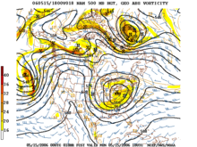
Forecast of surface pressures five days into the future for the North Pacific, North America, and the
North Atlantic OceanWeather forecasting is the application of science and technology to predict the conditions of the atmosphere for a given location and time. People have attempted to predict the weather informally for millennia and formally since the 19th century.
Weather forecasts are made by collecting quantitative data about the current state of the atmosphere, land, and ocean and using meteorology to project how the atmosphere will change at a given place.
Once calculated manually based mainly upon changes in barometric pressure, current weather conditions, and sky conditions or cloud cover, weather forecasting now relies on computer-based models that take many atmospheric factors into account.
Human input is still required to pick the best possible model to base
the forecast upon, which involves pattern recognition skills, teleconnections, knowledge of model performance, and knowledge of model biases.
The inaccuracy of forecasting is due to the chaotic
nature of the atmosphere, the massive computational power required to
solve the equations that describe the atmosphere, the land, and the
ocean, the error involved in measuring the initial conditions, and an
incomplete understanding of atmospheric and related processes. Hence,
forecasts become less accurate as the difference between current time
and the time for which the forecast is being made (the range of
the forecast) increases. The use of ensembles and model consensus helps
narrow the error and provide confidence in the forecast.
There is a vast variety of end uses for weather forecasts. Weather warnings are important because they are used to protect life and property. Forecasts based on temperature and precipitation
are important to agriculture, and therefore to traders within commodity
markets. Temperature forecasts are used by utility companies to
estimate demand over coming days.
On an everyday basis, many people use weather forecasts to
determine what to wear on a given day. Since outdoor activities are
severely curtailed by heavy rain, snow and wind chill, forecasts can be used to plan activities around these events, and to plan ahead and survive them.
Weather forecasting is a part of the economy. For example in
2009, the US spent approximately $5.8 billion on it, producing benefits
estimated at six times as much.
History
Ancient forecasting
For millennia, people have tried to forecast the weather. In 650 BC, the Babylonians predicted the weather from cloud patterns as well as astrology. In about 350 BC, Aristotle described weather patterns in Meteorologica. Later, Theophrastus compiled a book on weather forecasting, called the Book of Signs. Chinese weather prediction lore extends at least as far back as 300 BC, which was also around the same time ancient Indian astronomers developed weather-prediction methods. In New Testament
times, Jesus himself referred to deciphering and understanding local
weather patterns, by saying, "When evening comes, you say, 'It will be
fair weather, for the sky is red', and in the morning, 'Today it will be
stormy, for the sky is red and overcast.' You know how to interpret the
appearance of the sky, but you cannot interpret the signs of the
times."
In 904 AD, Ibn Wahshiyya's Nabatean Agriculture, translated into Arabic from an earlier Aramaic work,
discussed the weather forecasting of atmospheric changes and signs from
the planetary astral alterations; signs of rain based on observation of
the lunar phases; and weather forecasts based on the movement of winds.
Ancient weather forecasting methods usually relied on observed
patterns of events, also termed pattern recognition. For example, it was
observed that if the sunset was particularly red, the following day
often brought fair weather. This experience accumulated over the
generations to produce weather lore. However, not all of these predictions prove reliable, and many of them have since been found not to stand up to rigorous statistical testing.
Modern methods
The Royal Charter sank in an October 1859 storm, stimulating the establishment of modern weather forecasting.
It was not until the invention of the electric telegraph in 1835 that the modern age of weather forecasting began.
Before that, the fastest that distant weather reports could travel was
around 160 kilometres per day (100 mi/d), but was more typically 60–120
kilometres per day (40–75 mi/day) (whether by land or by sea). By the late 1840s, the telegraph allowed reports of weather conditions from a wide area to be received almost instantaneously, allowing forecasts to be made from knowledge of weather conditions further upwind.
The two men credited with the birth of forecasting as a science were an officer of the Royal Navy Francis Beaufort and his protégé Robert FitzRoy. Both were influential men in British
naval and governmental circles, and though ridiculed in the press at
the time, their work gained scientific credence, was accepted by the
Royal Navy, and formed the basis for all of today's weather forecasting
knowledge.
Beaufort developed the Wind Force Scale
and Weather Notation coding, which he was to use in his journals for
the remainder of his life. He also promoted the development of reliable
tide tables around British shores, and with his friend William Whewell, expanded weather record-keeping at 200 British coast guard stations.
Robert FitzRoy was appointed in 1854 as chief of a new department within the Board of Trade to deal with the collection of weather data at sea as a service to mariners. This was the forerunner of the modern Meteorological Office.
All ship captains were tasked with collating data on the weather and
computing it, with the use of tested instruments that were loaned for
this purpose.
Weather map of Europe, December 10, 1887
A storm in October 1859 that caused the loss of the Royal Charter inspired FitzRoy to develop charts to allow predictions to be made, which he called "forecasting the weather", thus coining the term "weather forecast". Fifteen land stations were established to use the telegraph
to transmit to him daily reports of weather at set times leading to the
first gale warning service. His warning service for shipping was
initiated in February 1861, with the use of telegraph communications. The first daily weather forecasts were published in The Times in 1861. In the following year a system was introduced of hoisting storm warning cones at the principal ports when a gale was expected. The "Weather Book" which FitzRoy published in 1863 was far in advance of the scientific opinion of the time.
As the electric telegraph network expanded, allowing for the more
rapid dissemination of warnings, a national observational network was
developed, which could then be used to provide synoptic analyses.
Instruments to continuously record variations in meteorological
parameters using photography were supplied to the observing stations from Kew Observatory – these cameras had been invented by Francis Ronalds in 1845 and his barograph had earlier been used by FitzRoy.
To convey accurate information, it soon became necessary to have a
standard vocabulary describing clouds; this was achieved by means of a
series of classifications first achieved by Luke Howard in 1802, and standardized in the International Cloud Atlas of 1896.
Numerical prediction
It was not until the 20th century that advances in the understanding of atmospheric physics led to the foundation of modern numerical weather prediction. In 1922, English scientist Lewis Fry Richardson published "Weather Prediction By Numerical Process",
after finding notes and derivations he worked on as an ambulance driver
in World War I. He described therein how small terms in the prognostic
fluid dynamics equations governing atmospheric flow could be neglected,
and a finite differencing scheme in time and space could be devised, to
allow numerical prediction solutions to be found.
Richardson envisioned a large auditorium of thousands of people
performing the calculations and passing them to others. However, the
sheer number of calculations required was too large to be completed
without the use of computers, and the size of the grid and time steps
led to unrealistic results in deepening systems. It was later found,
through numerical analysis, that this was due to numerical instability. The first computerised weather forecast was performed by a team composed of American meteorologists Jule Charney, Philip Duncan Thompson, Larry Gates, and Norwegian meteorologist Ragnar Fjørtoft, applied mathematician John von Neumann, and ENIAC programmer Klara Dan von Neumann. Practical use of numerical weather prediction began in 1955, spurred by the development of programmable electronic computers.
Broadcasts
The first ever daily weather forecasts were published in The Times on August 1, 1861, and the first weather maps were produced later in the same year. In 1911, the Met Office
began issuing the first marine weather forecasts via radio
transmission. These included gale and storm warnings for areas around
Great Britain. In the United States, the first public radio forecasts were made in 1925 by Edward B. "E.B." Rideout, on WEEI, the Edison Electric Illuminating station in Boston. Rideout came from the U.S. Weather Bureau, as did WBZ weather forecaster G. Harold Noyes in 1931.
BBC television weather chart for November 13, 1936
The world's first televised weather forecasts, including the use of weather maps, were experimentally broadcast by the BBC in November 1936. This was brought into practice in 1949, after World War II. George Cowling gave the first weather forecast while being televised in front of the map in 1954. In America, experimental television forecasts were made by James C. Fidler in Cincinnati in either 1940 or 1947 on the DuMont Television Network. In the late 1970s and early 1980s, John Coleman, the first weatherman for the American Broadcasting Company (ABC)'s Good Morning America, pioneered the use of on-screen weather satellite data and computer graphics for television forecasts. In 1982, Coleman partnered with Landmark Communications CEO Frank Batten to launch The Weather Channel
(TWC), a 24-hour cable network devoted to national and local weather
reports. Some weather channels have started broadcasting on live streaming platforms such as YouTube and Periscope to reach more viewers.
How models create forecasts
The basic idea of numerical weather prediction is to sample the state of the fluid at a given time and use the equations of fluid dynamics and thermodynamics
to estimate the state of the fluid at some time in the future. The main
inputs from country-based weather services are surface observations
from automated weather stations at ground level over land and from weather buoys at sea. The World Meteorological Organization
acts to standardize the instrumentation, observing practices and timing
of these observations worldwide. Stations either report hourly in METAR reports, or every six hours in SYNOP reports. Sites launch radiosondes, which rise through the depth of the troposphere and well into the stratosphere. Data from weather satellites are used in areas where traditional data sources are not available.
Compared with similar data from radiosondes, the satellite data has the
advantage of global coverage, but at a lower accuracy and resolution. Meteorological radar
provide information on precipitation location and intensity, which can
be used to estimate precipitation accumulations over time. Additionally, if a pulse Doppler weather radar is used then wind speed and direction can be determined.
These methods, however, leave an in-situ observational gap in the lower
atmosphere (from 100 m to 6 km above ground level). To reduce this gap,
in the late 1990s weather drones
started to be considered for obtaining data from those altitudes.
Research has been growing significantly since the 2010s, and
weather-drone data may in future be added to numerical weather models.
Modern weather predictions aid in timely evacuations and potentially save lives and prevent property damage
Commerce provides pilot reports along aircraft routes, and ship reports along shipping routes. Research flights using reconnaissance aircraft fly in and around weather systems of interest such as tropical cyclones.
Reconnaissance aircraft are also flown over the open oceans during the
cold season into systems that cause significant uncertainty in forecast
guidance, or are expected to be of high impact 3–7 days into the future
over the downstream continent.
Models are initialized using this observed data. The irregularly spaced observations are processed by data assimilation
and objective analysis methods, which perform quality control and
obtain values at locations usable by the model's mathematical algorithms
(usually an evenly spaced grid). The data are then used in the model as
the starting point for a forecast. Commonly, the set of equations used to predict the physics and dynamics of the atmosphere are called primitive equations.
These are initialized from the analysis data and rates of change are
determined. The rates of change predict the state of the atmosphere a
short time into the future. The equations are then applied to this new
atmospheric state to find new rates of change, which predict the
atmosphere at a yet further time into the future. This time stepping procedure is continually repeated until the solution reaches the desired forecast time.
The length of the time step chosen within the model is related to
the distance between the points on the computational grid, and is
chosen to maintain numerical stability. Time steps for global models are on the order of tens of minutes, while time steps for regional models are between one and four minutes. The global models are run at varying times into the future. The Met Office's Unified Model is run six days into the future, the European Centre for Medium-Range Weather Forecasts model is run out to 10 days into the future, while the Global Forecast System model run by the Environmental Modeling Center is run 16 days into the future. The visual output produced by a model solution is known as a prognostic chart, or prog.
The raw output is often modified before being presented as the
forecast. This can be in the form of statistical techniques to remove
known biases in the model, or of adjustment to take into account consensus among other numerical weather forecasts.
MOS or model output statistics is a technique used to interpret
numerical model output and produce site-specific guidance. This guidance
is presented in coded numerical form, and can be obtained for nearly
all National Weather Service reporting stations in the United States. As
proposed by Edward Lorenz
in 1963, long range forecasts, those made at a range of two weeks or
more cannot definitively predict the state of the atmosphere, owing to
the chaotic nature of the fluid dynamics
equations involved. In numerical models, extremely small errors in
initial values double roughly every five days for variables such as
temperature and wind velocity.
Essentially, a model is a computer program that produces meteorological
information for future times at given locations and altitudes. Within
any modern model is a set of equations, known as the primitive
equations, used to predict the future state of the atmosphere. These equations—along with the ideal gas law—are used to evolve the density, pressure, and potential temperature scalar fields and the velocity vector field of the atmosphere through time. Additional transport equations for pollutants and other aerosols are included in some primitive-equation mesoscale models as well. The equations used are nonlinear partial differential equations, which are impossible to solve exactly through analytical methods, with the exception of a few idealized cases.
Therefore, numerical methods obtain approximate solutions. Different
models use different solution methods: some global models use spectral methods for the horizontal dimensions and finite difference methods
for the vertical dimension, while regional and other global models
usually use finite-difference methods in all three dimensions.
Techniques
Persistence
The
simplest method of forecasting the weather, persistence, relies upon
today's conditions to forecast tomorrow's. This can be a valid way of
forecasting the weather when it is in a steady state, such as during the
summer season in the tropics. This method strongly depends upon the
presence of a stagnant weather pattern. Therefore, when in a fluctuating
pattern, it becomes inaccurate. It can be useful in both short- and
long-range forecast|long range forecasts.
Use of a barometer
Measurements
of barometric pressure and the pressure tendency (the change of
pressure over time) have been used in forecasting since the late 19th
century. The larger the change in pressure, especially if more than 3.5 hPa (2.6 mmHg), the larger the change in weather can be expected. If the pressure drop is rapid, a low pressure system is approaching, and there is a greater chance of rain. Rapid pressure rises are associated with improving weather conditions, such as clearing skies.
Looking at the sky
Marestail shows moisture at high altitude, signalling the later arrival of wet weather.
Along with pressure tendency, the condition of the sky is one of the
more important parameters used to forecast weather in mountainous areas.
Thickening of cloud cover or the invasion of a higher cloud deck is
indicative of rain in the near future. High thin cirrostratus clouds can create halos around the sun or moon, which indicates an approach of a warm front and its associated rain. Morning fog
portends fair conditions, as rainy conditions are preceded by wind or
clouds that prevent fog formation. The approach of a line of thunderstorms could indicate the approach of a cold front. Cloud-free skies are indicative of fair weather for the near future. A bar can indicate a coming tropical cyclone. The use of sky cover in weather prediction has led to various weather lore over the centuries.
Nowcasting
The forecasting of the weather within the next six hours is often referred to as nowcasting.
In this time range it is possible to forecast smaller features such as
individual showers and thunderstorms with reasonable accuracy, as well
as other features too small to be resolved by a computer model. A human
given the latest radar, satellite and observational data will be able to
make a better analysis of the small scale features present and so will
be able to make a more accurate forecast for the following few hours. However, there are now expert systems using those data and mesoscale numerical model to make better extrapolation, including evolution of those features in time. Accuweather is known for a Minute-Cast, which is a minute-by-minute precipitation forecast for the next two hours.
Use of forecast models
In the past, the human forecaster was responsible for generating the entire weather forecast based upon available observations. Today, human input is generally confined to choosing a model based on various parameters, such as model biases and performance. Using a consensus of forecast models, as well as ensemble members of the various models, can help reduce forecast error.
However, regardless how small the average error becomes with any
individual system, large errors within any particular piece of guidance
are still possible on any given model run.
Humans are required to interpret the model data into weather forecasts
that are understandable to the end user. Humans can use knowledge of
local effects that may be too small in size to be resolved by the model
to add information to the forecast. While increasing accuracy of
forecast models implies that humans may no longer be needed in the
forecast process at some point in the future, there is currently still a
need for human intervention.
Analog technique
The
analog technique is a complex way of making a forecast, requiring the
forecaster to remember a previous weather event that is expected to be
mimicked by an upcoming event. What makes it a difficult technique to
use is that there is rarely a perfect analog for an event in the future.
Some call this type of forecasting pattern recognition. It remains a
useful method of observing rainfall over data voids such as oceans,
as well as the forecasting of precipitation amounts and distribution in
the future. A similar technique is used in medium range forecasting,
which is known as teleconnections, when systems in other locations are
used to help pin down the location of another system within the
surrounding regime. An example of teleconnections are by using El Niño-Southern Oscillation (ENSO) related phenomena.
Communicating forecasts to the public

An example of a two-day weather forecast in the
visual style that an American newspaper might use. Temperatures are given in Fahrenheit.
Most end users of forecasts are members of the general public. Thunderstorms can create strong winds and dangerous lightning strikes that can lead to deaths, power outages, and widespread hail damage. Heavy snow or rain can bring transportation and commerce to a stand-still, as well as cause flooding in low-lying areas. Excessive heat or cold waves can sicken or kill those with inadequate utilities, and droughts can impact water usage and destroy vegetation.
Several countries employ government agencies to provide forecasts
and watches/warnings/advisories to the public to protect life and
property and maintain commercial interests. Knowledge of what the end
user needs from a weather forecast must be taken into account to present
the information in a useful and understandable way. Examples include
the National Oceanic and Atmospheric Administration's National Weather Service (NWS) and Environment Canada's Meteorological Service (MSC).
Traditionally, newspaper, television, and radio have been the primary
outlets for presenting weather forecast information to the public. In
addition, some cities had weather beacons. Increasingly, the internet is being used due to the vast amount of specific information that can be found. In all cases, these outlets update their forecasts on a regular basis.
Severe weather alerts and advisories
A
major part of modern weather forecasting is the severe weather alerts
and advisories that the national weather services issue in the case that
severe or hazardous weather is expected. This is done to protect life
and property. Some of the most commonly known of severe weather advisories are the severe thunderstorm and tornado warning, as well as the severe thunderstorm and tornado watch. Other forms of these advisories include winter weather, high wind, flood, tropical cyclone, and fog. Severe weather advisories and alerts are broadcast through the media, including radio, using emergency systems as the Emergency Alert System, which break into regular programming.
Low temperature forecast
The low temperature forecast for the current day is calculated using the lowest temperature found between 7 pm that evening through 7 am the following morning. So, in short, today's forecasted low is most likely tomorrow's low temperature.
Specialist forecasting
There
are a number of sectors with their own specific needs for weather
forecasts and specialist services are provided to these users as given
below:
Air traffic

Because the aviation industry is especially sensitive to the weather,
accurate weather forecasting is essential. Fog or exceptionally low ceilings can prevent many aircraft from landing and taking off. Turbulence and icing are also significant in-flight hazards. Thunderstorms are a problem for all aircraft because of severe turbulence due to their updrafts and outflow boundaries, icing due to the heavy precipitation, as well as large hail, strong winds, and lightning, all of which can cause severe damage to an aircraft in flight. Volcanic ash is also a significant problem for aviation, as aircraft can lose engine power within ash clouds. On a day-to-day basis airliners are routed to take advantage of the jet stream tailwind to improve fuel efficiency. Aircrews are briefed prior to takeoff on the conditions to expect en route and at their destination. Additionally, airports often change which runway is being used to take advantage of a headwind. This reduces the distance required for takeoff, and eliminates potential crosswinds.
Marine
Commercial and recreational use of waterways can be limited significantly by wind direction and speed, wave
periodicity and heights, tides, and precipitation. These factors can
each influence the safety of marine transit. Consequently, a variety of
codes have been established to efficiently transmit detailed marine
weather forecasts to vessel pilots via radio, for example the MAFOR (marine forecast). Typical weather forecasts can be received at sea through the use of RTTY, Navtex and Radiofax.
Agriculture
Farmers rely on weather forecasts to decide what work to do on any particular day. For example, drying hay is only feasible in dry weather. Prolonged periods of dryness can ruin cotton, wheat, and corn crops. While corn crops can be ruined by drought, their dried remains can be used as a cattle feed substitute in the form of silage. Frosts and freezes play havoc with crops both during the spring and fall. For example, peach trees in full bloom can have their potential peach crop decimated by a spring freeze. Orange groves can suffer significant damage during frosts and freezes, regardless of their timing.
Forestry
Forecasting of wind, precipitation and humidity is essential for preventing and controlling wildfires. Indices such as the Forest fire weather index and the Haines Index,
have been developed to predict the areas more at risk of fire from
natural or human causes. Conditions for the development of harmful
insects can also be predicted by forecasting the weather.
Utility companies
An
air handling unit is used for the heating and cooling of air in a central location (click on image for legend).
Electricity and gas companies rely on weather forecasts to anticipate
demand, which can be strongly affected by the weather. They use the
quantity termed the degree day to determine how strong of a use there
will be for heating (heating degree day)
or cooling (cooling degree day). These quantities are based on a daily
average temperature of 65 °F (18 °C). Cooler temperatures force heating
degree days (one per degree Fahrenheit), while warmer temperatures force
cooling degree days. In winter, severe cold weather can cause a surge in demand as people turn up their heating. Similarly, in summer a surge in demand can be linked with the increased use of air conditioning systems in hot weather.
By anticipating a surge in demand, utility companies can purchase
additional supplies of power or natural gas before the price increases,
or in some circumstances, supplies are restricted through the use of brownouts and blackouts.
Other commercial companies
Increasingly,
private companies pay for weather forecasts tailored to their needs so
that they can increase their profits or avoid large losses.
For example, supermarket chains may change the stocks on their shelves
in anticipation of different consumer spending habits in different
weather conditions. Weather forecasts can be used to invest in the
commodity market, such as futures in oranges, corn, soybeans, and oil.
Military applications
United Kingdom Armed Forces
Royal Navy
The UK Royal Navy, working with the UK Met Office,
has its own specialist branch of weather observers and forecasters, as
part of the Hydrographic and Meteorological (HM) specialisation, who
monitor and forecast operational conditions across the globe, to provide
accurate and timely weather and oceanographic information to
submarines, ships and Fleet Air Arm aircraft.
Royal Air Force
A mobile unit in the RAF,
working with the UK Met Office, forecasts the weather for regions in
which British, allied servicemen and women are deployed. A group based
at Camp Bastion provides forecasts for the British armed forces in Afghanistan.
United States Armed Forces
US Navy
Emblem of JTWC Joint Typhoon Warning Center
Similar to the private sector, military weather forecasters present
weather conditions to the war fighter community. Military weather
forecasters provide pre-flight and in-flight weather briefs to pilots
and provide real time resource protection services for military
installations. Naval forecasters cover the waters and ship weather
forecasts. The United States Navy
provides a special service to both themselves and the rest of the
federal government by issuing forecasts for tropical cyclones across the
Pacific and Indian Oceans through their Joint Typhoon Warning Center.
US Air Force
Within the United States, Air Force Weather provides weather forecasting for the Air Force and the Army.
Air Force forecasters cover air operations in both wartime and peacetime operations and provide
Army support;
United States Coast Guard marine science technicians provide ship forecasts for ice breakers and other various operations within their realm; and Marine forecasters provide support for ground- and air-based
United States Marine Corps operations. All four military branches take their initial enlisted meteorology technical training at
Keesler Air Force Base. Military and civilian forecasters actively cooperate in analyzing, creating and critiquing weather forecast products.

.svg)


.jpg)


