Matrix (mathematics)

From Wikipedia, the free encyclopedia

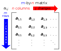
Each element of a matrix is often denoted by a variable with two subscripts. For instance, a_2,1 represents the element at the second row and first column of a matrix A.

In mathematics, a matrix (plural matrices) is a rectangular array^[1]—of numbers, symbols, or expressions, arranged in rows and columns^[2][3]—that is treated in certain prescribed ways. The individual items in a matrix are called its elements or entries. An example of a matrix with 2 rows and 3 columns is

Provided that they are the same size (have the same number of rows and the same number of columns), two matrices can be added or subtracted element by element. The rule for matrix multiplication, however, is that two matrices can be multiplied only when the number of columns in the first equals the number of rows in the second. A major application of matrices is to represent linear transformations, that is, generalizations of linear functions such as f(x) = 4x. For example, the rotation of vectors in three dimensional space is a linear transformation which can be represented by a rotation matrix R: if v is a column vector (a matrix with only one column) describing the position of a point in space, the product Rv is a column vector describing the position of that point after a rotation. The product of two transformation matrices is a matrix that represents the composition of two linear transformations.
Another application of matrices is in the solution of systems of linear equations. If the matrix is square, it is possible to deduce some of its properties by computing its determinant. For example, a square matrix has an inverse if and only if its determinant is not zero. Insight into the geometry of a linear transformation is obtainable (along with other information) from the matrix's eigenvalues and eigenvectors.

Applications of matrices are found in most scientific fields. In every branch of physics, including classical mechanics, optics, electromagnetism, quantum mechanics, and quantum electrodynamics, they are used to study physical phenomena, such as the motion of rigid bodies. In computer graphics, they are used to project a 3-dimensional image onto a 2-dimensional screen. In probability theory and statistics, stochastic matrices are used to describe sets of probabilities; for instance, they are used within the PageRank algorithm that ranks the pages in a Google search.^[4] Matrix calculus generalizes classical analytical notions such as derivatives and exponentials to higher dimensions.

A major branch of numerical analysis is devoted to the development of efficient algorithms for matrix computations, a subject that is centuries old and is today an expanding area of research. Matrix decomposition methods simplify computations, both theoretically and practically. Algorithms that are tailored to particular matrix structures, such as sparse matrices and near-diagonal matrices, expedite computations in finite element method and other computations. Infinite matrices occur in planetary theory and in atomic theory. A simple example of an infinite matrix is the matrix representing the derivative operator, which acts on the Taylor series of a function.

Definition

A matrix is a rectangular array of numbers or other mathematical objects, for which operations such as addition and multiplication are defined.^[5] Most commonly, a matrix over a field F is a rectangular array of scalars from F.^[6][7] Most of this article focuses on real and complex matrices, i.e., matrices whose elements are real numbers or complex numbers, respectively. More general types of entries are discussed below. For instance, this is a real matrix:

The numbers, symbols or expressions in the matrix are called its entries or its elements. The horizontal and vertical lines of entries in a matrix are called rows and columns, respectively.

Size

The size of a matrix is defined by the number of rows and columns that it contains. A matrix with m rows and n columns is called an m × n matrix or m-by-n matrix, while m and n are called its dimensions. For example, the matrix A above is a 3 × 2 matrix.

Matrices which have a single row are called row vectors, and those which have a single column are called column vectors. A matrix which has the same number of rows and columns is called a square matrix. A matrix with an infinite number of rows or columns (or both) is called an infinite matrix. In some contexts, such as computer algebra programs, it is useful to consider a matrix with no rows or no columns, called an empty matrix.

Name	Size	Example	Description
Row vector	1 × n		A matrix with one row, sometimes used to represent a vector
Column vector	n × 1		A matrix with one column, sometimes used to represent a vector
Square matrix	n × n		A matrix with the same number of rows and columns, sometimes used to represent a linear transformation from a vector space to itself, such as reflection, rotation, or shearing.

Notation

Matrices are commonly written in box brackets:

An alternative notation uses large parentheses instead of box brackets:

The specifics of symbolic matrix notation varies widely, with some prevailing trends. Matrices are usually symbolized using upper-case letters (such as A in the examples above), while the corresponding lower-case letters, with two subscript indices (e.g., a₁₁, or a_1,1), represent the entries. In addition to using upper-case letters to symbolize matrices, many authors use a special typographical style, commonly boldface upright (non-italic), to further distinguish matrices from other mathematical objects. An alternative notation involves the use of a double-underline with the variable name, with or without boldface style, (e.g., ).

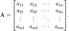
The entry in the i-th row and j-th column of a matrix A is sometimes referred to as the i,j, (i,j), or (i,j)^th entry of the matrix, and most commonly denoted as a_i,j, or a_ij. Alternative notations for that entry are A[i,j] or A_i,j. For example, the (1,3) entry of the following matrix A is 5 (also denoted a₁₃, a_1,3, A[1,3] or A_1,3):

Sometimes, the entries of a matrix can be defined by a formula such as a_i,j = f(i, j). For example, each of the entries of the following matrix A is determined by a_ij = i − j.

In this case, the matrix itself is sometimes defined by that formula, within square brackets or double parenthesis. For example, the matrix above is defined as A = [i-j], or A = ((i-j)). If matrix size is m × n, the above-mentioned formula f(i, j) is valid for any i = 1, ..., m and any j = 1, ..., n. This can be either specified separately, or using m × n as a subscript. For instance, the matrix A above is 3 × 4 and can be defined as A = [i − j] (i = 1, 2, 3; j = 1, ..., 4), or A = [i − j]_3×4.

Some programming languages utilize doubly subscripted arrays (or arrays of arrays) to represent an m-×-n matrix. Some programming languages start the numbering of array indexes at zero, in which case the entries of an m-by-n matrix are indexed by 0 ≤ i ≤ m − 1 and 0 ≤ j ≤ n − 1.^[8] This article follows the more common convention in mathematical writing where enumeration starts from 1.

The set of all m-by-n matrices is denoted 𝕄(m, n).

Basic operations

There are a number of basic operations that can be applied to modify matrices, called matrix addition, scalar multiplication, transposition, matrix multiplication, row operations, and submatrix.^[10]

Addition, scalar multiplication and transposition

Operation	Definition	Example
Addition	The sum A+B of two m-by-n matrices A and B is calculated entrywise: (A + B)i,j = Ai,j + Bi,j, where 1 ≤ i ≤ m and 1 ≤ j ≤ n.
Scalar multiplication	The product cA of a number c (also called a scalar in the parlance of abstract algebra) and a matrix A is computed by multiplying every entry of A by c: (cA)i,j = c · Ai,j. This operation is called scalar multiplication, but its result is not named “scalar product” to avoid confusion, since “scalar product” is sometimes used as a synonym for “inner product”.
Transposition	The transpose of an m-by-n matrix A is the n-by-m matrix AT (also denoted Atr or tA) formed by turning rows into columns and vice versa: (AT)i,j = Aj,i.

Familiar properties of numbers extend to these operations of matrices: for example, addition is commutative, i.e., the matrix sum does not depend on the order of the summands: A + B = B + A.^[11] The transpose is compatible with addition and scalar multiplication, as expressed by (cA)^T = c(A^T) and (A + B)^T = A^T + B^T. Finally, (A^T)^T = A.

Matrix multiplication

Schematic depiction of the matrix product AB of two matrices A and B.

Multiplication of two matrices is defined if and only if the number of columns of the left matrix is the same as the number of rows of the right matrix. If A is an m-by-n matrix and B is an n-by-p matrix, then their matrix product AB is the m-by-p matrix whose entries are given by dot product of the corresponding row of A and the corresponding column of B:

,

where 1 ≤ i ≤ m and 1 ≤ j ≤ p.^[12] For example, the underlined entry 2340 in the product is calculated as (2 × 1000) + (3 × 100) + (4 × 10) = 2340:

Matrix multiplication satisfies the rules (AB)C = A(BC) (associativity), and (A+B)C = AC+BC as well as C(A+B) = CA+CB (left and right distributivity), whenever the size of the matrices is such that the various products are defined.^[13] The product AB may be defined without BA being defined, namely if A and B are m-by-n and n-by-k matrices, respectively, and m ≠ k. Even if both products are defined, they need not be equal, i.e., generally

AB ≠ BA,

i.e., matrix multiplication is not commutative, in marked contrast to (rational, real, or complex) numbers whose product is independent of the order of the factors. An example of two matrices not commuting with each other is:

whereas

Besides the ordinary matrix multiplication just described, there exist other less frequently used operations on matrices that can be considered forms of multiplication, such as the Hadamard product and the Kronecker product.^[14] They arise in solving matrix equations such as the Sylvester equation.

Row operations

There are three types of row operations:

1. row addition, that is adding a row to another.
2. row multiplication, that is multiplying all entries of a row by a non-zero constant;
3. row switching, that is interchanging two rows of a matrix;

These operations are used in a number of ways, including solving linear equations and finding matrix inverses.

Submatrix

A submatrix of a matrix is obtained by deleting any collection of rows and/or columns.^[15][16][17] For example, from the following 3-by-4 matrix, we can construct a 2-by-3 submatrix by removing row 3 and column 2:

The minors and cofactors of a matrix are found by computing the determinant of certain submatrices.^[17][18]

A principal submatrix is a square submatrix obtained by removing certain rows and columns. The definition varies from author to author. According to some authors, a principal submatrix is a submatrix in which the set of row indices that remain is the same as the set of column indices that remain.^[19][20] Other authors define a principal submatrix to be one in which the first k rows and columns, for some number k, are the ones that remain;^[21] this type of submatrix has also been called a leading principal submatrix.^[22]

Linear equations

Matrices can be used to compactly write and work with multiple linear equations, i.e., systems of linear equations. For example, if A is an m-by-n matrix, x designates a column vector (i.e., n×1-matrix) of n variables x₁, x₂, ..., x_n, and b is an m×1-column vector, then the matrix equation

Ax = b

is equivalent to the system of linear equations

A_1,1x₁ + A_1,2x₂ + ... + A_1,nx_n = b₁

...

A_m,1x₁ + A_m,2x₂ + ... + A_m,nx_n = b_m .^[23]

Linear transformations

The vectors represented by a 2-by-2 matrix correspond to the sides of a unit square transformed into a parallelogram.

Matrices and matrix multiplication reveal their essential features when related to linear transformations, also known as linear maps. A real m-by-n matrix A gives rise to a linear transformation Rⁿ → R^m mapping each vector x in Rⁿ to the (matrix) product Ax, which is a vector in R^m. Conversely, each linear transformation f: Rⁿ → R^m arises from a unique m-by-n matrix A: explicitly, the (i, j)-entry of A is the i^th coordinate of f(e_j), where e_j = (0,...,0,1,0,...,0) is the unit vector with 1 in the j^th position and 0 elsewhere. The matrix A is said to represent the linear map f, and A is called the transformation matrix of f.
For example, the 2×2 matrix

can be viewed as the transform of the unit square into a parallelogram with vertices at (0, 0), (a, b), (a + c, b + d), and (c, d). The parallelogram pictured at the right is obtained by multiplying A with each of the column vectors and in turn. These vectors define the vertices of the unit square.

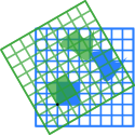
The following table shows a number of 2-by-2 matrices with the associated linear maps of R². The blue original is mapped to the green grid and shapes. The origin (0,0) is marked with a black point.

Horizontal shear with m=1.25.	Horizontal flip	Squeeze mapping with r=3/2	Scaling by a factor of 3/2	Rotation by π/6R = 30°

Under the 1-to-1 correspondence between matrices and linear maps, matrix multiplication corresponds to composition of maps:^[24] if a k-by-m matrix B represents another linear map g : R^m → R^k, then the composition g ∘ f is represented by BA since

(g ∘ f)(x) = g(f(x)) = g(Ax) = B(Ax) = (BA)x.

The last equality follows from the above-mentioned associativity of matrix multiplication.

The rank of a matrix A is the maximum number of linearly independent row vectors of the matrix, which is the same as the maximum number of linearly independent column vectors.^[25] Equivalently it is the dimension of the image of the linear map represented by A.^[26] The rank-nullity theorem states that the dimension of the kernel of a matrix plus the rank equals the number of columns of the matrix.^[27]

Square matrices

A square matrix is a matrix with the same number of rows and columns. An n-by-n matrix is known as a square matrix of order n. Any two square matrices of the same order can be added and multiplied. The entries a_ii form the main diagonal of a square matrix. They lie on the imaginary line which runs from the top left corner to the bottom right corner of the matrix.

Main types

Name	Example with n = 3
Diagonal matrix
Lower triangular matrix
Upper triangular matrix

Diagonal and triangular matrices

If all entries of A below the main diagonal are zero, A is called an upper triangular matrix. Similarly if all entries of A above the main diagonal are zero, A is called a lower triangular matrix. If all entries outside the main diagonal are zero, A is called a diagonal matrix.

Identity matrix[edit]

The identity matrix I_n of size n is the n-by-n matrix in which all the elements on the main diagonal are equal to 1 and all other elements are equal to 0, e.g.

It is a square matrix of order n, and also a special kind of diagonal matrix. It is called identity matrix because multiplication with it leaves a matrix unchanged:

AI_n = I_mA = A for any m-by-n matrix A.

Symmetric or skew-symmetric matrix

A square matrix A that is equal to its transpose, i.e., A = A^T, is a symmetric matrix. If instead, A was equal to the negative of its transpose, i.e., A = −A^T, then A is a skew-symmetric matrix. In complex matrices, symmetry is often replaced by the concept of Hermitian matrices, which satisfy A^∗ = A, where the star or asterisk denotes the conjugate transpose of the matrix, i.e., the transpose of the complex conjugate of A.

By the spectral theorem, real symmetric matrices and complex Hermitian matrices have an eigenbasis; i.e., every vector is expressible as a linear combination of eigenvectors. In both cases, all eigenvalues are real.^[28] This theorem can be generalized to infinite-dimensional situations related to matrices with infinitely many rows and columns, see below.

Invertible matrix and its inverse

A square matrix A is called invertible or non-singular if there exists a matrix B such that

AB = BA = I_n.^[29][30]

If B exists, it is unique and is called the inverse matrix of A, denoted A⁻¹.

Definite matrix

Positive definite matrix	Indefinite matrix
Q(x,y) = 1/4 x2 + y2	Q(x,y) = 1/4 x2 − 1/4 y2
Points such that Q(x,y)=1 (Ellipse).	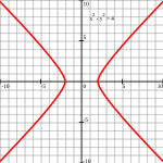Points such that Q(x,y)=1 (Hyperbola).

A symmetric n×n-matrix is called positive-definite (respectively negative-definite; indefinite), if for all nonzero vectors x ∈ Rⁿ the associated quadratic form given by

Q(x) = x^TAx

takes only positive values (respectively only negative values; both some negative and some positive values).^[31] If the quadratic form takes only non-negative (respectively only non-positive) values, the symmetric matrix is called positive-semidefinite (respectively negative-semidefinite); hence the matrix is indefinite precisely when it is neither positive-semidefinite nor negative-semidefinite.

A symmetric matrix is positive-definite if and only if all its eigenvalues are positive, i.e., the matrix is positive-semidefinite and it is invertible.^[32] The table at the right shows two possibilities for 2-by-2 matrices.

Allowing as input two different vectors instead yields the bilinear form associated to A:

B_A (x, y) = x^TAy.^[33]

Orthogonal matrix

An orthogonal matrix is a square matrix with real entries whose columns and rows are orthogonal unit vectors (i.e., orthonormal vectors). Equivalently, a matrix A is orthogonal if its transpose is equal to its inverse:

which entails

where I is the identity matrix.

An orthogonal matrix A is necessarily invertible (with inverse A⁻¹ = A^T), unitary (A⁻¹ = A*), and normal (A*A = AA*). The determinant of any orthogonal matrix is either +1 or −1. A special orthogonal matrix is an orthogonal matrix with determinant +1. As a linear transformation, every orthogonal matrix with determinant +1 is a pure rotation, while every orthogonal matrix with determinant -1 is either a pure reflection, or a composition of reflection and rotation.

The complex analogue of an orthogonal matrix is a unitary matrix.

Main operations

Trace

The trace, tr(A) of a square matrix A is the sum of its diagonal entries. While matrix multiplication is not commutative as mentioned above, the trace of the product of two matrices is independent of the order of the factors:

tr(AB) = tr(BA).

This is immediate from the definition of matrix multiplication:

Also, the trace of a matrix is equal to that of its transpose, i.e.,

tr(A) = tr(A^T).

Determinant

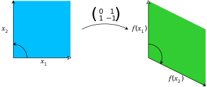
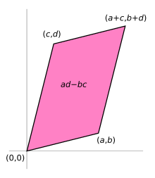
A linear transformation on R² given by the indicated matrix. The determinant of this matrix is −1, as the area of the green parallelogram at the right is 1, but the map reverses the orientation, since it turns the counterclockwise orientation of the vectors to a clockwise one.

The determinant det(A) or |A| of a square matrix A is a number encoding certain properties of the matrix. A matrix is invertible if and only if its determinant is nonzero. Its absolute value equals the area (in R²) or volume (in R³) of the image of the unit square (or cube), while its sign corresponds to the orientation of the corresponding linear map: the determinant is positive if and only if the orientation is preserved.

The determinant of 2-by-2 matrices is given by

The determinant of 3-by-3 matrices involves 6 terms (rule of Sarrus). The more lengthy Leibniz formula generalises these two formulae to all dimensions.^[34]

The determinant of a product of square matrices equals the product of their determinants:

det(AB) = det(A) · det(B).^[35]

Adding a multiple of any row to another row, or a multiple of any column to another column, does not change the determinant. Interchanging two rows or two columns affects the determinant by multiplying it by −1.^[36] Using these operations, any matrix can be transformed to a lower (or upper) triangular matrix, and for such matrices the determinant equals the product of the entries on the main diagonal; this provides a method to calculate the determinant of any matrix. Finally, the Laplace expansion expresses the determinant in terms of minors, i.e., determinants of smaller matrices.^[37] This expansion can be used for a recursive definition of determinants (taking as starting case the determinant of a 1-by-1 matrix, which is its unique entry, or even the determinant of a 0-by-0 matrix, which is 1), that can be seen to be equivalent to the Leibniz formula. Determinants can be used to solve linear systems using Cramer's rule, where the division of the determinants of two related square matrices equates to the value of each of the system's variables.^[38]

Eigenvalues and eigenvectors

A number λ and a non-zero vector v satisfying

Av = λv

are called an eigenvalue and an eigenvector of A, respectively.^{[nb 1][39]} The number λ is an eigenvalue of an n×n-matrix A if and only if A−λI_n is not invertible, which is equivalent to

^[40]

The polynomial p_A in an indeterminate X given by evaluation the determinant det(XI_n−A) is called the characteristic polynomial of A. It is a monic polynomial of degree n. Therefore the polynomial equation p_A(λ) = 0 has at most n different solutions, i.e., eigenvalues of the matrix.^[41] They may be complex even if the entries of A are real.
According to the Cayley–Hamilton theorem, p_A(A) = 0, that is, the result of substituting the matrix itself into its own characteristic polynomial yields the zero matrix.

Computational aspects

Matrix calculations can be often performed with different techniques. Many problems can be solved by both direct algorithms or iterative approaches. For example, the eigenvectors of a square matrix can be obtained by finding a sequence of vectors x_n converging to an eigenvector when n tends to infinity.^[42]

To be able to choose the more appropriate algorithm for each specific problem, it is important to determine both the effectiveness and precision of all the available algorithms. The domain studying these matters is called numerical linear algebra.^[43] As with other numerical situations, two main aspects are the complexity of algorithms and their numerical stability.

Determining the complexity of an algorithm means finding upper bounds or estimates of how many elementary operations such as additions and multiplications of scalars are necessary to perform some algorithm, e.g., multiplication of matrices. For example, calculating the matrix product of two n-by-n matrix using the definition given above needs n³ multiplications, since for any of the n² entries of the product, n multiplications are necessary. The Strassen algorithm outperforms this "naive" algorithm; it needs only n^2.807 multiplications.^[44] A refined approach also incorporates specific features of the computing devices.

In many practical situations additional information about the matrices involved is known. An important case are sparse matrices, i.e., matrices most of whose entries are zero. There are specifically adapted algorithms for, say, solving linear systems Ax = b for sparse matrices A, such as the conjugate gradient method.^[45]

An algorithm is, roughly speaking, numerically stable, if little deviations in the input values do not lead to big deviations in the result. For example, calculating the inverse of a matrix via Laplace's formula (Adj (A) denotes the adjugate matrix of A)

A⁻¹ = Adj(A) / det(A)

may lead to significant rounding errors if the determinant of the matrix is very small. The norm of a matrix can be used to capture the conditioning of linear algebraic problems, such as computing a matrix's inverse.^[46]

Although most computer languages are not designed with commands or libraries for matrices, as early as the 1970s, some engineering desktop computers such as the HP 9830 had ROM cartridges to add BASIC commands for matrices. Some computer languages such as APL were designed to manipulate matrices, and various mathematical programs can be used to aid computing with matrices.^[47]

Decomposition

There are several methods to render matrices into a more easily accessible form. They are generally referred to as matrix decomposition or matrix factorization techniques. The interest of all these techniques is that they preserve certain properties of the matrices in question, such as determinant, rank or inverse, so that these quantities can be calculated after applying the transformation, or that certain matrix operations are algorithmically easier to carry out for some types of matrices.
The LU decomposition factors matrices as a product of lower (L) and an upper triangular matrices (U).^[48] Once this decomposition is calculated, linear systems can be solved more efficiently, by a simple technique called forward and back substitution. Likewise, inverses of triangular matrices are algorithmically easier to calculate. The Gaussian elimination is a similar algorithm; it transforms any matrix to row echelon form.^[49] Both methods proceed by multiplying the matrix by suitable elementary matrices, which correspond to permuting rows or columns and adding multiples of one row to another row. Singular value decomposition expresses any matrix A as a product UDV^∗, where U and V are unitary matrices and D is a diagonal matrix.

An example of a matrix in Jordan normal form. The grey blocks are called Jordan blocks.

The eigendecomposition or diagonalization expresses A as a product VDV⁻¹, where D is a diagonal matrix and V is a suitable invertible matrix.^[50] If A can be written in this form, it is called diagonalizable. More generally, and applicable to all matrices, the Jordan decomposition transforms a matrix into Jordan normal form, that is to say matrices whose only nonzero entries are the eigenvalues λ₁ to λ_n of A, placed on the main diagonal and possibly entries equal to one directly above the main diagonal, as shown at the right.^[51] Given the eigendecomposition, the n^th power of A (i.e., n-fold iterated matrix multiplication) can be calculated via

Aⁿ = (VDV⁻¹)ⁿ = VDV⁻¹VDV⁻¹...VDV⁻¹ = VDⁿV⁻¹

and the power of a diagonal matrix can be calculated by taking the corresponding powers of the diagonal entries, which is much easier than doing the exponentiation for A instead. This can be used to compute the matrix exponential e^A, a need frequently arising in solving linear differential equations, matrix logarithms and square roots of matrices.^[52] To avoid numerically ill-conditioned situations, further algorithms such as the Schur decomposition can be employed.^[53]

Abstract algebraic aspects and generalizations

Matrices can be generalized in different ways. Abstract algebra uses matrices with entries in more general fields or even rings, while linear algebra codifies properties of matrices in the notion of linear maps. It is possible to consider matrices with infinitely many columns and rows. Another extension are tensors, which can be seen as higher-dimensional arrays of numbers, as opposed to vectors, which can often be realised as sequences of numbers, while matrices are rectangular or two-dimensional arrays of numbers.^[54] Matrices, subject to certain requirements tend to form groups known as matrix groups.

Matrices with more general entries

This article focuses on matrices whose entries are real or complex numbers. However, matrices can be considered with much more general types of entries than real or complex numbers. As a first step of generalization, any field, i.e., a set where addition, subtraction, multiplication and division operations are defined and well-behaved, may be used instead of R or C, for example rational numbers or finite fields. For example, coding theory makes use of matrices over finite fields. Wherever eigenvalues are considered, as these are roots of a polynomial they may exist only in a larger field than that of the entries of the matrix; for instance they may be complex in case of a matrix with real entries. The possibility to reinterpret the entries of a matrix as elements of a larger field (e.g., to view a real matrix as a complex matrix whose entries happen to be all real) then allows considering each square matrix to possess a full set of eigenvalues. Alternatively one can consider only matrices with entries in an algebraically closed field, such as C, from the outset.

More generally, abstract algebra makes great use of matrices with entries in a ring R.^[55] Rings are a more general notion than fields in that a division operation need not exist. The very same addition and multiplication operations of matrices extend to this setting, too. The set M(n, R) of all square n-by-n matrices over R is a ring called matrix ring, isomorphic to the endomorphism ring of the left R-module Rⁿ.^[56] If the ring R is commutative, i.e., its multiplication is commutative, then M(n, R) is a unitary noncommutative (unless n = 1) associative algebra over R.
The determinant of square matrices over a commutative ring R can still be defined using the Leibniz formula; such a matrix is invertible if and only if its determinant is invertible in R, generalising the situation over a field F, where every nonzero element is invertible.^[57] Matrices over superrings are called supermatrices.^[58]

Matrices do not always have all their entries in the same ring – or even in any ring at all. One special but common case is block matrices, which may be considered as matrices whose entries themselves are matrices. The entries need not be quadratic matrices, and thus need not be members of any ordinary ring; but their sizes must fulfil certain compatibility conditions.

Relationship to linear maps

Linear maps Rⁿ → R^m are equivalent to m-by-n matrices, as described above. More generally, any linear map f: V → W between finite-dimensional vector spaces can be described by a matrix A = (a_ij), after choosing bases v₁, ..., v_n of V, and w₁, ..., w_m of W (so n is the dimension of V and m is the dimension of W), which is such that

In other words, column j of A expresses the image of v_j in terms of the basis vectors w_i of W; thus this relation uniquely determines the entries of the matrix A. Note that the matrix depends on the choice of the bases: different choices of bases give rise to different, but equivalent matrices.^[59] Many of the above concrete notions can be reinterpreted in this light, for example, the transpose matrix A^T describes the transpose of the linear map given by A, with respect to the dual bases.^[60]

These properties can be restated in a more natural way: the category of all matrices with entries in a field with multiplication as composition is equivalent to the category of finite dimensional vector spaces and linear maps over this field.

More generally, the set of m×n matrices can be used to represent the R-linear maps between the free modules R^m and Rⁿ for an arbitrary ring R with unity. When n = m composition of these maps is possible, and this gives rise to the matrix ring of n×n matrices representing the endomorphism ring of Rⁿ.

Matrix groups

A group is a mathematical structure consisting of a set of objects together with a binary operation, i.e., an operation combining any two objects to a third, subject to certain requirements.^[61] A group in which the objects are matrices and the group operation is matrix multiplication is called a matrix group.^{[nb 2][62]} Since in a group every element has to be invertible, the most general matrix groups are the groups of all invertible matrices of a given size, called the general linear groups.
Any property of matrices that is preserved under matrix products and inverses can be used to define further matrix groups. For example, matrices with a given size and with a determinant of 1 form a subgroup of (i.e., a smaller group contained in) their general linear group, called a special linear group.^[63] Orthogonal matrices, determined by the condition

M^TM = I,

form the orthogonal group.^[64] Every orthogonal matrix has determinant 1 or −1. Orthogonal matrices with determinant 1 form a subgroup called special orthogonal group.

Every finite group is isomorphic to a matrix group, as one can see by considering the regular representation of the symmetric group.^[65] General groups can be studied using matrix groups, which are comparatively well-understood, by means of representation theory.^[66]

Infinite matrices

It is also possible to consider matrices with infinitely many rows and/or columns^[67] even if, being infinite objects, one cannot write down such matrices explicitly. All that matters is that for every element in the set indexing rows, and every element in the set indexing columns, there is a well-defined entry (these index sets need not even be subsets of the natural numbers). The basic operations of addition, subtraction, scalar multiplication and transposition can still be defined without problem; however matrix multiplication may involve infinite summations to define the resulting entries, and these are not defined in general.
If R is any ring with unity, then the ring of endomorphisms of as a right R module is isomorphic to the ring of column finite matrices whose entries are indexed by , and whose columns each contain only finitely many nonzero entries. The endomorphisms of M considered as a left R module result in an analogous object, the row finite matrices whose rows each only have finitely many nonzero entries.

If infinite matrices are used to describe linear maps, then only those matrices can be used all of whose columns have but a finite number of nonzero entries, for the following reason. For a matrix A to describe a linear map f: V→W, bases for both spaces must have been chosen; recall that by definition this means that every vector in the space can be written uniquely as a (finite) linear combination of basis vectors, so that written as a (column) vector v of coefficients, only finitely many entries v_i are nonzero. Now the columns of A describe the images by f of individual basis vectors of V in the basis of W, which is only meaningful if these columns have only finitely many nonzero entries. There is no restriction on the rows of A however: in the product A·v there are only finitely many nonzero coefficients of v involved, so every one of its entries, even if it is given as an infinite sum of products, involves only finitely many nonzero terms and is therefore well defined. Moreover this amounts to forming a linear combination of the columns of A that effectively involves only finitely many of them, whence the result has only finitely many nonzero entries, because each of those columns do. One also sees that products of two matrices of the given type is well defined (provided as usual that the column-index and row-index sets match), is again of the same type, and corresponds to the composition of linear maps.

If R is a normed ring, then the condition of row or column finiteness can be relaxed. With the norm in place, absolutely convergent series can be used instead of finite sums. For example, the matrices whose column sums are absolutely convergent sequences form a ring. Analogously of course, the matrices whose row sums are absolutely convergent series also form a ring.

In that vein, infinite matrices can also be used to describe operators on Hilbert spaces, where convergence and continuity questions arise, which again results in certain constraints that have to be imposed. However, the explicit point of view of matrices tends to obfuscate the matter,^{[nb 3]} and the abstract and more powerful tools of functional analysis can be used instead.

Empty matrices

An empty matrix is a matrix in which the number of rows or columns (or both) is zero.^[68][69] Empty matrices help dealing with maps involving the zero vector space. For example, if A is a 3-by-0 matrix and B is a 0-by-3 matrix, then AB is the 3-by-3 zero matrix corresponding to the null map from a 3-dimensional space V to itself, while BA is a 0-by-0 matrix. There is no common notation for empty matrices, but most computer algebra systems allow creating and computing with them. The determinant of the 0-by-0 matrix is 1 as follows from regarding the empty product occurring in the Leibniz formula for the determinant as 1. This value is also consistent with the fact that the identity map from any finite dimensional space to itself has determinant 1, a fact that is often used as a part of the characterization of determinants.

Applications

There are numerous applications of matrices, both in mathematics and other sciences. Some of them merely take advantage of the compact representation of a set of numbers in a matrix. For example, in game theory and economics, the payoff matrix encodes the payoff for two players, depending on which out of a given (finite) set of alternatives the players choose.^[70] Text mining and automated thesaurus compilation makes use of document-term matrices such as tf-idf to track frequencies of certain words in several documents.^[71]

Complex numbers can be represented by particular real 2-by-2 matrices via

under which addition and multiplication of complex numbers and matrices correspond to each other. For example, 2-by-2 rotation matrices represent the multiplication with some complex number of absolute value 1, as above. A similar interpretation is possible for quaternions^[72] and Clifford algebras in general.

Early encryption techniques such as the Hill cipher also used matrices. However, due to the linear nature of matrices, these codes are comparatively easy to break.^[73] Computer graphics uses matrices both to represent objects and to calculate transformations of objects using affine rotation matrices to accomplish tasks such as projecting a three-dimensional object onto a two-dimensional screen, corresponding to a theoretical camera observation.^[74] Matrices over a polynomial ring are important in the study of control theory.

Chemistry makes use of matrices in various ways, particularly since the use of quantum theory to discuss molecular bonding and spectroscopy. Examples are the overlap matrix and the Fock matrix used in solving the Roothaan equations to obtain the molecular orbitals of the Hartree–Fock method.

Graph theory

An undirected graph with adjacency matrix

The adjacency matrix of a finite graph is a basic notion of graph theory.^[75] It records which vertices of the graph are connected by an edge. Matrices containing just two different values (1 and 0 meaning for example "yes" and "no", respectively) are called logical matrices. The distance (or cost) matrix contains information about distances of the edges.^[76] These concepts can be applied to websites connected by hyperlinks or cities connected by roads etc., in which case (unless the connection network is extremely dense) the matrices tend to be sparse, i.e., contain few nonzero entries. Therefore, specifically tailored matrix algorithms can be used in network theory.

Analysis and geometry

The Hessian matrix of a differentiable function ƒ: Rⁿ → R consists of the second derivatives of ƒ with respect to the several coordinate directions, i.e.^[77]

At the saddle point (x = 0, y = 0) (red) of the function f(x,−y) = x² − y², the Hessian matrix is indefinite.

It encodes information about the local growth behaviour of the function: given a critical point x = (x₁, ..., x_n), i.e., a point where the first partial derivatives of ƒ vanish, the function has a local minimum if the Hessian matrix is positive definite. Quadratic programming can be used to find global minima or maxima of quadratic functions closely related to the ones attached to matrices (see above).^[78]

Another matrix frequently used in geometrical situations is the Jacobi matrix of a differentiable map f: Rⁿ → R^m. If f₁, ..., f_m denote the components of f, then the Jacobi matrix is defined as ^[79]

If n < m, and if the rank of the Jacobi matrix attains its maximal value m, f is locally invertible at that point, by the implicit function theorem.^[80]

Partial differential equations can be classified by considering the matrix of coefficients of the highest-order differential operators of the equation. For elliptic partial differential equations this matrix is positive definite, which has decisive influence on the set of possible solutions of the equation in question.^[81]

The finite element method is an important numerical method to solve partial differential equations, widely applied in simulating complex physical systems. It attempts to approximate the solution to some equation by piecewise linear functions, where the pieces are chosen with respect to a sufficiently fine grid, which in turn can be recast as a matrix equation.^[82]

Probability theory and statistics

Two different Markov chains. The chart depicts the number of particles (of a total of 1000) in state "2". Both limiting values can be determined from the transition matrices, which are given by (red) and (black).

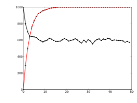
Stochastic matrices are square matrices whose rows are probability vectors, i.e., whose entries are non-negative and sum up to one. Stochastic matrices are used to define Markov chains with finitely many states.^[83] A row of the stochastic matrix gives the probability distribution for the next position of some particle currently in the state that corresponds to the row. Properties of the Markov chain like absorbing states, i.e., states that any particle attains eventually, can be read off the eigenvectors of the transition matrices.^[84]

Statistics also makes use of matrices in many different forms.^[85] Descriptive statistics is concerned with describing data sets, which can often be represented as data matrices, which may then be subjected to dimensionality reduction techniques. The covariance matrix encodes the mutual variance of several random variables.^[86] Another technique using matrices are linear least squares, a method that approximates a finite set of pairs (x₁, y₁), (x₂, y₂), ..., (x_N, y_N), by a linear function

y_i ≈ ax_i + b, i = 1, ..., N

which can be formulated in terms of matrices, related to the singular value decomposition of matrices.^[87]

Random matrices are matrices whose entries are random numbers, subject to suitable probability distributions, such as matrix normal distribution. Beyond probability theory, they are applied in domains ranging from number theory to physics.^[88][89]

Symmetries and transformations in physics

Linear transformations and the associated symmetries play a key role in modern physics. For example, elementary particles in quantum field theory are classified as representations of the Lorentz group of special relativity and, more specifically, by their behavior under the spin group. Concrete representations involving the Pauli matrices and more general gamma matrices are an integral part of the physical description of fermions, which behave as spinors.^[90] For the three lightest quarks, there is a group-theoretical representation involving the special unitary group SU(3); for their calculations, physicists use a convenient matrix representation known as the Gell-Mann matrices, which are also used for the SU(3) gauge group that forms the basis of the modern description of strong nuclear interactions, quantum chromodynamics. The Cabibbo–Kobayashi–Maskawa matrix, in turn, expresses the fact that the basic quark states that are important for weak interactions are not the same as, but linearly related to the basic quark states that define particles with specific and distinct masses.^[91]

Linear combinations of quantum states

The first model of quantum mechanics (Heisenberg, 1925) represented the theory's operators by infinite-dimensional matrices acting on quantum states.^[92] This is also referred to as matrix mechanics. One particular example is the density matrix that characterizes the "mixed" state of a quantum system as a linear combination of elementary, "pure" eigenstates.^[93]

Another matrix serves as a key tool for describing the scattering experiments that form the cornerstone of experimental particle physics: Collision reactions such as occur in particle accelerators, where non-interacting particles head towards each other and collide in a small interaction zone, with a new set of non-interacting particles as the result, can be described as the scalar product of outgoing particle states and a linear combination of ingoing particle states. The linear combination is given by a matrix known as the S-matrix, which encodes all information about the possible interactions between particles.^[94]

Normal modes

A general application of matrices in physics is to the description of linearly coupled harmonic systems. The equations of motion of such systems can be described in matrix form, with a mass matrix multiplying a generalized velocity to give the kinetic term, and a force matrix multiplying a displacement vector to characterize the interactions. The best way to obtain solutions is to determine the system's eigenvectors, its normal modes, by diagonalizing the matrix equation. Techniques like this are crucial when it comes to the internal dynamics of molecules: the internal vibrations of systems consisting of mutually bound component atoms.^[95] They are also needed for describing mechanical vibrations, and oscillations in electrical circuits.^[96]

Geometrical optics

Geometrical optics provides further matrix applications. In this approximative theory, the wave nature of light is neglected. The result is a model in which light rays are indeed geometrical rays. If the deflection of light rays by optical elements is small, the action of a lens or reflective element on a given light ray can be expressed as multiplication of a two-component vector with a two-by-two matrix called ray transfer matrix: the vector's components are the light ray's slope and its distance from the optical axis, while the matrix encodes the properties of the optical element. Actually, there are two kinds of matrices, viz. a refraction matrix describing the refraction at a lens surface, and a translation matrix, describing the translation of the plane of reference to the next refracting surface, where another refraction matrix applies. The optical system, consisting of a combination of lenses and/or reflective elements, is simply described by the matrix resulting from the product of the components' matrices.^[97]

Electronics

Traditional mesh analysis in electronics leads to a system of linear equations that can be described with a matrix.
The behaviour of many electronic components can be described using matrices. Let A be a 2-dimensional vector with the component's input voltage v₁ and input current i₁ as its elements, and let B be a 2-dimensional vector with the component's output voltage v₂ and output current i₂ as its elements. Then the behaviour of the electronic component can be described by B = H · A, where H is a 2 x 2 matrix containing one impedance element (h₁₂), one admittance element (h₂₁) and two dimensionless elements (h₁₁ and h₂₂). Calculating a circuit now reduces to multiplying matrices.

History

Matrices have a long history of application in solving linear equations but they were known as arrays until the 1800s. The Chinese text The Nine Chapters on the Mathematical Art written in 10th–2nd century BCE is the first example of the use of array methods to solve simultaneous equations,^[98] including the concept of determinants. In 1545 Italian mathematician Girolamo Cardano brought the method to Europe when he published Ars Magna.^[99] The Japanese mathematician Seki used the same array methods to solve simultaneous equations in 1683.^[100] The Dutch Mathematician Jan de Witt represented transformations using arrays in his 1659 book Elements of Curves (1659).^[101] Between 1700 and 1710 Gottfried Wilhelm Leibniz publicized the use of arrays for recording information or solutions and experimented with over 50 different systems of arrays.^[99] Cramer presented his rule in 1750.

The term "matrix" (Latin for "womb", derived from mater—mother^[102]) was coined by James Joseph Sylvester in 1850,^[103] who understood a matrix as an object giving rise to a number of determinants today called minors, that is to say, determinants of smaller matrices that derive from the original one by removing columns and rows. In an 1851 paper, Sylvester explains:

I have in previous papers defined a "Matrix" as a rectangular array of terms, out of which different systems of determinants may be engendered as from the womb of a common parent.^[104]

Arthur Cayley published a treatise on geometric transformations using matrices that were not rotated versions of the coefficients being investigated as had previously been done. Instead he defined operations such as addition, subtraction, multiplication, and division as transformations of those matrices and showed the associative and distributive properties held true. Cayley investigated and demonstrated the non-commutative property of matrix multiplication as well as the commutative property of matrix addition.^[99] Early matrix theory had limited the use of arrays almost exclusively to determinants and Arthur Cayley's abstract matrix operations were revolutionary. He was instrumental in proposing a matrix concept independent of equation systems. In 1858 Cayley published his Memoir on the theory of matrices^[105][106] in which he proposed and demonstrated the Cayley-Hamilton theorem.^[99]

An English mathematician named Cullis was the first to use modern bracket notation for matrices in 1913 and he simultaneously demonstrated the first significant use the notation A = [a_i,j] to represent a matrix where a_i,j refers to the ith row and the jth column.^[99]

The study of determinants sprang from several sources.^[107] Number-theoretical problems led Gauss to relate coefficients of quadratic forms, i.e., expressions such as x² + xy − 2y², and linear maps in three dimensions to matrices. Eisenstein further developed these notions, including the remark that, in modern parlance, matrix products are non-commutative. Cauchy was the first to prove general statements about determinants, using as definition of the determinant of a matrix A = [a_i,j] the following: replace the powers a_j^k by a_jk in the polynomial

,

where Π denotes the product of the indicated terms. He also showed, in 1829, that the eigenvalues of symmetric matrices are real.^[108] Jacobi studied "functional determinants"—later called Jacobi determinants by Sylvester—which can be used to describe geometric transformations at a local (or infinitesimal) level, see above; Kronecker's Vorlesungen über die Theorie der Determinanten^[109] and Weierstrass' Zur Determinantentheorie,^[110] both published in 1903, first treated determinants axiomatically, as opposed to previous more concrete approaches such as the mentioned formula of Cauchy. At that point, determinants were firmly established.

Many theorems were first established for small matrices only, for example the Cayley–Hamilton theorem was proved for 2×2 matrices by Cayley in the aforementioned memoir, and by Hamilton for 4×4 matrices. Frobenius, working on bilinear forms, generalized the theorem to all dimensions (1898). Also at the end of the 19th century the Gauss–Jordan elimination (generalizing a special case now known as Gauss elimination) was established by Jordan. In the early 20th century, matrices attained a central role in linear algebra.^[111] partially due to their use in classification of the hypercomplex number systems of the previous century.

The inception of matrix mechanics by Heisenberg, Born and Jordan led to studying matrices with infinitely many rows and columns.^[112] Later, von Neumann carried out the mathematical formulation of quantum mechanics, by further developing functional analytic notions such as linear operators on Hilbert spaces, which, very roughly speaking, correspond to Euclidean space, but with an infinity of independent directions.

Other historical usages of the word “matrix” in mathematics

The word has been used in unusual ways by at least two authors of historical importance.

Bertrand Russell and Alfred North Whitehead in their Principia Mathematica (1910–1913) use the word “matrix” in the context of their Axiom of reducibility. They proposed this axiom as a means to reduce any function to one of lower type, successively, so that at the “bottom” (0 order) the function is identical to its extension:

“Let us give the name of matrix to any function, of however many variables, which does not involve any apparent variables. Then any possible function other than a matrix is derived from a matrix by means of generalization, i.e., by considering the proposition which asserts that the function in question is true with all possible values or with some value of one of the arguments, the other argument or arguments remaining undetermined”.^[113]

For example a function Φ(x, y) of two variables x and y can be reduced to a collection of functions of a single variable, e.g., y, by “considering” the function for all possible values of “individuals” a_i substituted in place of variable x. And then the resulting collection of functions of the single variable y, i.e., ∀a_i: Φ(a_i, y), can be reduced to a “matrix” of values by “considering” the function for all possible values of “individuals” b_i substituted in place of variable y:

∀b_j∀a_i: Φ(a_i, b_j).

Alfred Tarski in his 1946 Introduction to Logic used the word “matrix” synonymously with the notion of truth table as used in mathematical logic.^[114]