Negative feedback

From Wikipedia, the free encyclopedia

https://en.wikipedia.org/wiki/Negative_feedback

A simple negative feedback system is descriptive, for example, of some electronic amplifiers. The feedback is negative if the loop gain AB is negative.

Negative feedback (or balancing feedback) occurs when some function of the output of a system, process, or mechanism is fed back in a manner that tends to reduce the fluctuations in the output, whether caused by changes in the input or by other disturbances.

Whereas positive feedback tends to instability via exponential growth, oscillation or chaotic behavior, negative feedback generally promotes stability. Negative feedback tends to promote a settling to equilibrium, and reduces the effects of perturbations. Negative feedback loops in which just the right amount of correction is applied with optimum timing, can be very stable, accurate, and responsive.

Negative feedback is widely used in mechanical and electronic engineering, and it is observed in many other fields including biology, chemistry and economics. General negative feedback systems are studied in control systems engineering.

Negative feedback loops also play an integral role in maintaining the atmospheric balance in various climate systems on Earth. One such feedback system is the interaction between solar radiation, cloud cover, and planet temperature.

Blood glucose levels are maintained at a constant level in the body by a negative feedback mechanism. When the blood glucose level is too high, the pancreas secretes insulin and when the level is too low, the pancreas then secretes glucagon. The flat line shown represents the homeostatic set point. The sinusoidal line represents the blood glucose level.

General description

Feedback loops in the human body

In many physical and biological systems, qualitatively different influences can oppose each other. For example, in biochemistry, one set of chemicals drives the system in a given direction, whereas another set of chemicals drives it in an opposing direction. If one or both of these opposing influences are non-linear, equilibrium point(s) result.

In biology, this process (in general, biochemical) is often referred to as homeostasis; whereas in mechanics, the more common term is equilibrium.

In engineering, mathematics and the physical, and biological sciences, common terms for the points around which the system gravitates include: attractors, stable states, eigenstates/eigenfunctions, equilibrium points, and setpoints.

In control theory, negative refers to the sign of the multiplier in mathematical models for feedback. In delta notation, −Δoutput is added to or mixed into the input. In multivariate systems, vectors help to illustrate how several influences can both partially complement and partially oppose each other.

Some authors, in particular with respect to modelling business systems, use negative to refer to the reduction in difference between the desired and actual behavior of a system. In a psychology context, on the other hand, negative refers to the valence of the feedback – attractive versus aversive, or praise versus criticism.

In contrast, positive feedback is feedback in which the system responds so as to increase the magnitude of any particular perturbation, resulting in amplification of the original signal instead of stabilization. Any system in which there is positive feedback together with a gain greater than one will result in a runaway situation. Both positive and negative feedback require a feedback loop to operate.

However, negative feedback systems can still be subject to oscillations. This is caused by a phase shift around any loop. Due to these phase shifts the feedback signal of some frequencies can ultimately become in phase with the input signal and thus turn into positive feedback, creating a runaway condition. Even before the point where the phase shift becomes 180 degrees, stability of the negative feedback loop will become compromised, leading to increasing under- and overshoot following a disturbance. This problem is often dealt with by attenuating or changing the phase of the problematic frequencies in a design step called compensation. Unless the system naturally has sufficient damping, many negative feedback systems have low pass filters or dampers fitted.

Examples

• Mercury thermostats (circa 1600) using expansion and contraction of columns of mercury in response to temperature changes were used in negative feedback systems to control vents in furnaces, maintaining a steady internal temperature.
• In the invisible hand of the market metaphor of economic theory (1776), reactions to price movements provide a feedback mechanism to match supply and demand.
• In centrifugal governors (1788), negative feedback is used to maintain a near-constant speed of an engine, irrespective of the load or fuel-supply conditions.
• In a steering engine (1866), power assistance is applied to the rudder with a feedback loop, to maintain the direction set by the steersman.
• In servomechanisms, the speed or position of an output, as determined by a sensor, is compared to a set value, and any error is reduced by negative feedback to the input.
• In audio amplifiers, negative feedback flattens frequency response, reduces distortion, minimises the effect of manufacturing variations in component parameters, and compensates for changes in characteristics due to temperature change.
• In analog computing, feedback around operational amplifiers is used to generate mathematical functions such as addition, subtraction, integration, differentiation, logarithm, and antilog functions.
• In delta-sigma analog-to-digital and digital-to-analog converters (particularly for high quality audio), a negative feedback loop is used to repeatedly correct accumulated quantization error during conversion.
• In a phase locked loop (1932), feedback is used to maintain a generated alternating waveform in a constant phase to a reference signal. In many implementations the generated waveform is the output, but when used as a demodulator in an FM radio receiver, the error feedback voltage serves as the demodulated output signal. If there is a frequency divider between the generated waveform and the phase comparator, the device acts as a frequency multiplier.
• In organisms, feedback enables various measures (e.g. body temperature, or blood sugar level) to be maintained within a desired range by homeostatic processes.

Detailed implementations

Error-controlled regulation

Basic error-controlled regulator loop

See also: Control engineering, Homeostasis, and Allostasis

A regulator R adjusts the input to a system T so the monitored essential variables E are held to set-point values S that result in the desired system output despite disturbances D.

One use of feedback is to make a system (say T) self-regulating to minimize the effect of a disturbance (say D). Using a negative feedback loop, a measurement of some variable (for example, a process variable, say E) is subtracted from a required value (the 'set point') to estimate an operational error in system status, which is then used by a regulator (say R) to reduce the gap between the measurement and the required value. The regulator modifies the input to the system T according to its interpretation of the error in the status of the system. This error may be introduced by a variety of possible disturbances or 'upsets', some slow and some rapid. The regulation in such systems can range from a simple 'on-off' control to a more complex processing of the error signal.

In this framework, the physical form of a signal may undergo multiple transformations. For example, a change in weather may cause a disturbance to the heat input to a house (as an example of the system T) that is monitored by a thermometer as a change in temperature (as an example of an 'essential variable' E). This quantity, then, is converted by the thermostat (a 'comparator') into an electrical error in status compared to the 'set point' S, and subsequently used by the regulator (containing a 'controller' that commands gas control valves and an ignitor) ultimately to change the heat provided by a furnace (an 'effector') to counter the initial weather-related disturbance in heat input to the house.

Error controlled regulation is typically carried out using a Proportional-Integral-Derivative Controller (PID controller). The regulator signal is derived from a weighted sum of the error signal, integral of the error signal, and derivative of the error signal. The weights of the respective components depend on the application.

Mathematically, the regulator signal is given by:

${\displaystyle \mathrm{M}\mathrm{V}(\mathrm{t})=K_p\left(e(t)+\frac{1}{T_i}{\int }_0^{t}e(\tau )d\tau +T_d\frac{d}{dt}e(t)\right)}$

where

${\displaystyle T_i}$ is the integral time

${\displaystyle T_d}$ is the derivative time

Negative feedback amplifier

Main article: Negative-feedback amplifier

The negative feedback amplifier was invented by Harold Stephen Black at Bell Laboratories in 1927, and granted a patent in 1937 (US Patent 2,102,671) "a continuation of application Serial No. 298,155, filed August 8, 1928 ...").

"The patent is 52 pages long plus 35 pages of figures. The first 43 pages amount to a small treatise on feedback amplifiers!"

There are many advantages to feedback in amplifiers. In design, the type of feedback and amount of feedback are carefully selected to weigh and optimize these various benefits.

Advantages of amplifier negative voltage feedback

Negative voltage feedback in amplifiers has the following advantages; it

1. reduces non-linear distortion, i.e., produces higher fidelity;
2. increases circuit stability: i.e., gains remain stable over variations in ambient temperature, frequency, and signal amplitude;
3. slightly increases bandwidth;
4. modifies input and output impedances;
5. considerably reduces harmonic, phase, amplitude, and frequency distortions; and
6. considerably reduces noise.

Though negative feedback has many advantages, amplifiers with feedback can oscillate (see Step response of feedback amplifiers), and they may exhibit instability. Harry Nyquist of Bell Laboratories proposed the a stability criterion and a plot to identify stable feedback systems, including amplifiers and control systems.

Negative feedback amplifier with external disturbance. The feedback is negative if βA >0.

The figure shows a simplified block diagram of a negative feedback amplifier.

The feedback sets the overall (closed-loop) amplifier gain at a value:

${\displaystyle \frac{O}{I}=\frac{A}{1+\beta A}\approx \frac{1}{\beta },}$

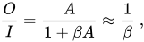
where the approximate value assumes βA >> 1. This expression shows that a gain greater than one requires β < 1. Because the approximate gain 1/β is independent of the open-loop gain A, the feedback is said to 'desensitize' the closed-loop gain to variations in A (for example, due to manufacturing variations between units, or temperature effects upon components), provided only that the gain A is sufficiently large. In this context, the factor (1+βA) is often called the 'desensitivity factor', and in the broader context of feedback effects that include other matters like electrical impedance and bandwidth, the 'improvement factor'.

If the disturbance D is included, the amplifier output becomes:

${\displaystyle O=\frac{AI}{1+\beta A}+\frac{D}{1+\beta A},}$

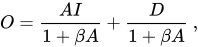
which shows that the feedback reduces the effect of the disturbance by the 'improvement factor' (1+β A). The disturbance D might arise from fluctuations in the amplifier output due to noise and nonlinearity (distortion) within this amplifier, or from other noise sources such as power supplies.

The difference signal I–βO at the amplifier input is sometimes called the "error signal". According to the diagram, the error signal is:

${\displaystyle \text{Error signal}=I-\beta O=I\left(1-\beta \frac{O}{I}\right)=\frac{I}{1+\beta A}-\frac{\beta D}{1+\beta A}.}$

From this expression, it can be seen that a large 'improvement factor' (or a large loop gain βA) tends to keep this error signal small.

Although the diagram illustrates the principles of the negative feedback amplifier, modeling a real amplifier as a unilateral forward amplification block and a unilateral feedback block has significant limitations. For methods of analysis that do not make these idealizations, see the article Negative feedback amplifier.

Operational amplifier circuits

Main article: Operational amplifier applications

A feedback voltage amplifier using an op amp with finite gain but infinite input impedances and zero output impedance.

The operational amplifier was originally developed as a building block for the construction of analog computers, but is now used almost universally in all kinds of applications including audio equipment and control systems.

Operational amplifier circuits typically employ negative feedback to get a predictable transfer function. Since the open-loop gain of an op-amp is extremely large, a small differential input signal would drive the output of the amplifier to one rail or the other in the absence of negative feedback. A simple example of the use of feedback is the op-amp voltage amplifier shown in the figure.

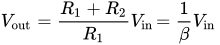
The idealized model of an operational amplifier assumes that the gain is infinite, the input impedance is infinite, output resistance is zero, and input offset currents and voltages are zero. Such an ideal amplifier draws no current from the resistor divider. Ignoring dynamics (transient effects and propagation delay), the infinite gain of the ideal op-amp means this feedback circuit drives the voltage difference between the two op-amp inputs to zero. Consequently, the voltage gain of the circuit in the diagram, assuming an ideal op amp, is the reciprocal of feedback voltage division ratio β:

${\displaystyle V_{\text{out}}=\frac{R_{\text{1}}+R_{\text{2}}}{R_{\text{1}}}{V}_{\text{in}}=\frac{1}{\beta }{V}_{\text{in}}}$.

A real op-amp has a high but finite gain A at low frequencies, decreasing gradually at higher frequencies. In addition, it exhibits a finite input impedance and a non-zero output impedance. Although practical op-amps are not ideal, the model of an ideal op-amp often suffices to understand circuit operation at low enough frequencies. As discussed in the previous section, the feedback circuit stabilizes the closed-loop gain and desensitizes the output to fluctuations generated inside the amplifier itself.

Areas of application

Mechanical engineering

See also: Control systems and Control engineering

The ballcock or float valve uses negative feedback to control the water level in a cistern.

An example of the use of negative feedback control is the ballcock control of water level (see diagram), or a pressure regulator. In modern engineering, negative feedback loops are found in engine governors, fuel injection systems and carburettors. Similar control mechanisms are used in heating and cooling systems, such as those involving air conditioners, refrigerators, or freezers.

Biology

See also: Counterregulatory hormone and Homeostasis

Control of endocrine hormones by negative feedback.

Some biological systems exhibit negative feedback such as the baroreflex in blood pressure regulation and erythropoiesis. Many biological processes (e.g., in the human anatomy) use negative feedback. Examples of this are numerous, from the regulating of body temperature, to the regulating of blood glucose levels. The disruption of feedback loops can lead to undesirable results: in the case of blood glucose levels, if negative feedback fails, the glucose levels in the blood may begin to rise dramatically, thus resulting in diabetes.

For hormone secretion regulated by the negative feedback loop: when gland X releases hormone X, this stimulates target cells to release hormone Y. When there is an excess of hormone Y, gland X "senses" this and inhibits its release of hormone X. As shown in the figure, most endocrine hormones are controlled by a physiologic negative feedback inhibition loop, such as the glucocorticoids secreted by the adrenal cortex. The hypothalamus secretes corticotropin-releasing hormone, which directs the anterior pituitary gland to secrete adrenocorticotropic hormone (ACTH). In turn, ACTH directs the adrenal cortex to secrete glucocorticoids, such as cortisol. Glucocorticoids not only perform their respective functions throughout the body but also negatively affect the release of further stimulating secretions of both the hypothalamus and the pituitary gland, effectively reducing the output of glucocorticoids once a sufficient amount has been released.

Chemistry

Closed systems containing substances undergoing a reversible chemical reaction can also exhibit negative feedback in accordance with Le Chatelier's principle which shift the chemical equilibrium to the opposite side of the reaction in order to reduce a stress. For example, in the reaction

N₂ + 3 H₂ ⇌ 2 NH₃ + 92 kJ/mol

If a mixture of the reactants and products exists at equilibrium in a sealed container and nitrogen gas is added to this system, then the equilibrium will shift toward the product side in response. If the temperature is raised, then the equilibrium will shift toward the reactant side which, since the reverse reaction is endothermic, will partially reduce the temperature.

Self-organization

Main articles: Self-organization and Emergence

Self-organization is the capability of certain systems "of organizing their own behavior or structure". There are many possible factors contributing to this capacity, and most often positive feedback is identified as a possible contributor. However, negative feedback also can play a role.

Economics

In economics, automatic stabilisers are government programs that are intended to work as negative feedback to dampen fluctuations in real GDP.

Mainstream economics asserts that the market pricing mechanism operates to match supply and demand, because mismatches between them feed back into the decision-making of suppliers and demanders of goods, altering prices and thereby reducing any discrepancy. However Norbert Wiener wrote in 1948:

"There is a belief current in many countries and elevated to the rank of an official article of faith in the United States that free competition is itself a homeostatic process... Unfortunately the evidence, such as it is, is against this simple-minded theory."

The notion of economic equilibrium being maintained in this fashion by market forces has also been questioned by numerous heterodox economists such as financier George Soros and leading ecological economist and steady-state theorist Herman Daly, who was with the World Bank in 1988–1994.

Environmental science

Some effects of climate change can either enhance (positive feedbacks) or weaken (negative feedbacks) global warming.

A basic and common example of a negative feedback system in the environment is the interaction among cloud cover, plant growth, solar radiation, and planet temperature. As incoming solar radiation increases, planet temperature increases. As the temperature increases, the amount of plant life that can grow increases. This plant life can then make products such as sulfur which produce more cloud cover. An increase in cloud cover leads to higher albedo, or surface reflectivity, of the Earth. As albedo increases, however, the amount of solar radiation decreases. This, in turn, affects the rest of the cycle.

Cloud cover, and in turn planet albedo and temperature, is also influenced by the hydrological cycle. As planet temperature increases, more water vapor is produced, creating more clouds. The clouds then block incoming solar radiation, lowering the temperature of the planet. This interaction produces less water vapor and therefore less cloud cover. The cycle then repeats in a negative feedback loop. In this way, negative feedback loops in the environment have a stabilizing effect.

History

Negative feedback as a control technique may be seen in the refinements of the water clock introduced by Ktesibios of Alexandria in the 3rd century BCE. Self-regulating mechanisms have existed since antiquity, and were used to maintain a constant level in the reservoirs of water clocks as early as 200 BCE.

The fly-ball governor, an early example of negative feedback

Negative feedback was implemented in the 17th century. Cornelius Drebbel had built thermostatically controlled incubators and ovens in the early 1600s, and centrifugal governors were used to regulate the distance and pressure between millstones in windmills. James Watt patented a form of governor in 1788 to control the speed of his steam engine, and James Clerk Maxwell in 1868 described "component motions" associated with these governors that lead to a decrease in a disturbance or the amplitude of an oscillation.

The term "feedback" was well established by the 1920s, in reference to a means of boosting the gain of an electronic amplifier. Friis and Jensen described this action as "positive feedback" and made passing mention of a contrasting "negative feed-back action" in 1924. Harold Stephen Black came up with the idea of using negative feedback in electronic amplifiers in 1927, submitted a patent application in 1928, and detailed its use in his paper of 1934, where he defined negative feedback as a type of coupling that reduced the gain of the amplifier, in the process greatly increasing its stability and bandwidth.

Karl Küpfmüller published papers on a negative-feedback-based automatic gain control system and a feedback system stability criterion in 1928.

Nyquist and Bode built on Black's work to develop a theory of amplifier stability.

Early researchers in the area of cybernetics subsequently generalized the idea of negative feedback to cover any goal-seeking or purposeful behavior.

All purposeful behavior may be considered to require negative feed-back. If a goal is to be attained, some signals from the goal are necessary at some time to direct the behavior.

Cybernetics pioneer Norbert Wiener helped to formalize the concepts of feedback control, defining feedback in general as "the chain of the transmission and return of information", and negative feedback as the case when:

The information fed back to the control center tends to oppose the departure of the controlled from the controlling quantity...^: 97

While the view of feedback as any "circularity of action" helped to keep the theory simple and consistent, Ashby pointed out that, while it may clash with definitions that require a "materially evident" connection, "the exact definition of feedback is nowhere important". Ashby pointed out the limitations of the concept of "feedback":

The concept of 'feedback', so simple and natural in certain elementary cases, becomes artificial and of little use when the interconnections between the parts become more complex...Such complex systems cannot be treated as an interlaced set of more or less independent feedback circuits, but only as a whole. For understanding the general principles of dynamic systems, therefore, the concept of feedback is inadequate in itself. What is important is that complex systems, richly cross-connected internally, have complex behaviors, and that these behaviors can be goal-seeking in complex patterns.^: 54

To reduce confusion, later authors have suggested alternative terms such as degenerative, self-correcting, balancing, or discrepancy-reducing in place of "negative".

False vacuum

From Wikipedia, the free encyclopedia

https://en.wikipedia.org/wiki/False_vacuum 

A scalar field φ (which represents physical position) in a false vacuum. The energy E is higher in the false vacuum than that in the true vacuum or ground state, but there is a barrier preventing the field from classically rolling down to the true vacuum. Therefore, the transition to the true vacuum must be stimulated by the creation of high-energy particles or through quantum-mechanical tunneling.

In quantum field theory, a false vacuum is a hypothetical vacuum state that is locally stable but does not occupy the most stable possible ground state. In this condition it is called metastable. It may last for a very long time in this state, but could eventually decay to the more stable one, an event known as false vacuum decay. The most common suggestion of how such a decay might happen in our universe is called bubble nucleation‌—if a small region of the universe by chance reached a more stable vacuum, this "bubble" (also called "bounce") would spread.

A false vacuum exists at a local minimum of energy and is therefore not completely stable, in contrast to a true vacuum, which exists at a global minimum and is stable.

Definition of true vs. false vacuum

A vacuum is defined as a space with as little energy in it as possible. Despite the name, the vacuum still has quantum fields. A true vacuum is stable because it is at a global minimum of energy, and is commonly assumed to coincide with the physical vacuum state in which we live. It is possible that a physical vacuum state is a configuration of quantum fields representing a local minimum but not global minimum of energy. This type of vacuum state is called a "false vacuum".

Implications

Existential threat

If our universe is in a false vacuum state rather than a true vacuum state, then the decay from the less stable false vacuum to the more stable true vacuum (called false vacuum decay) could have dramatic consequences. The effects could range from complete cessation of existing fundamental forces, elementary particles and structures comprising them, to subtle change in some cosmological parameters, mostly depending on the potential difference between true and false vacuum. Some false vacuum decay scenarios are compatible with the survival of structures like galaxies, stars, and even biological life, while others involve the full destruction of baryonic matter or even immediate gravitational collapse of the universe. In this more extreme case, the likelihood of a "bubble" forming is very low (i.e. one in 10⁸⁶⁸ or false vacuum decay may even be impossible).

A paper by Coleman and De Luccia that attempted to include simple gravitational assumptions into these theories noted that if this was an accurate representation of nature, then the resulting universe "inside the bubble" in such a case would appear to be extremely unstable and would almost immediately collapse:

In general, gravitation makes the probability of vacuum decay smaller; in the extreme case of minimal energy-density difference, it can even stabilize the false vacuum, preventing vacuum decay altogether. We believe we understand this. For the vacuum to decay, building a bubble of total energy zero must be possible. In the absence of gravitation, this is no problem, no matter how small the energy-density difference; all one has to do is make the bubble big enough, and the volume/surface ratio will do the job. In the presence of gravitation, though, the negative energy density of the true vacuum distorts geometry within the bubble with the result that, for a small enough energy density, there is no bubble with a big enough volume/surface ratio. Within the bubble, the effects of gravitation are more dramatic. The geometry of space-time within the bubble is that of anti-de Sitter space, a space much like conventional de Sitter space except that its group of symmetries is O(3, 2) rather than O(4, 1). Although this space-time is free of singularities, it is unstable under small perturbations, and inevitably suffers gravitational collapse of the same sort as the end state of a contracting Friedmann universe. The time required for the collapse of the interior universe is on the order of ... microseconds or less.

The possibility that we are living in a false vacuum has never been a cheering one to contemplate. Vacuum decay is the ultimate ecological catastrophe; in the new vacuum there are new constants of nature; after vacuum decay, not only is life as we know it impossible, so is chemistry as we know it. Nonetheless, one could always draw stoic comfort from the possibility that perhaps over time the new vacuum would sustain if not life as we know it, at least some structures capable of knowing joy. This possibility has now been eliminated.

The second special case is decay into a space of vanishing cosmological constant, the case that applies if we are now living in the debris of a false vacuum that decayed at some early cosmic epoch. This case presents us with less interesting physics and with fewer occasions for rhetorical excess than the preceding one. It is now the interior of the bubble that is ordinary Minkowski space ...

— Sidney Coleman and Frank De Luccia

In a 2005 paper published in Nature, as part of their investigation into global catastrophic risks, MIT physicist Max Tegmark and Oxford philosopher Nick Bostrom calculate the natural risks of the destruction of the Earth at less than 1/10⁹ per year from all natural (i.e. non-anthropogenic) events, including a transition to a lower vacuum state. They argue that due to observer selection effects, we might underestimate the chances of being destroyed by vacuum decay because any information about this event would reach us only at the instant when we too were destroyed. This is in contrast to events like risks from impacts, gamma-ray bursts, supernovae and hypernovae, the frequencies of which we have adequate direct measures.

Inflation

A number of theories suggest that cosmic inflation may be an effect of a false vacuum decaying into the true vacuum. The inflation itself may be the consequence of the Higgs field trapped in a false vacuum state with Higgs self-coupling λ and its β_λ function very close to zero at the planck scale. A future electron-positron collider would be able to provide the precise measurements of the top quark needed for such calculations.

Chaotic inflation theory suggests that the universe may be in either a false vacuum or a true vacuum state. Alan Guth, in his original proposal for cosmic inflation, proposed that inflation could end through quantum mechanical bubble nucleation of the sort described above. See history of Chaotic inflation theory. It was soon understood that a homogeneous and isotropic universe could not be preserved through the violent tunneling process. This led Andrei Linde and, independently, Andreas Albrecht and Paul Steinhardt, to propose "new inflation" or "slow roll inflation" in which no tunnelling occurs, and the inflationary scalar field instead graphs as a gentle slope.

In 2014, researchers at the Chinese Academy of Sciences' Wuhan Institute of Physics and Mathematics gave an actual mathematical demonstration of the already existing idea that the universe could have been spontaneously created from nothing (no space, time, nor matter) by quantum fluctuations of a metastable false vacuum causing an expanding bubble of true vacuum.

Vacuum decay varieties

Electroweak vacuum decay

Electroweak vacuum stability landscape as estimated in 2012

Electroweak vacuum stability landscape as estimated in 2018. T_RH is grand unification energy. ξ is the degree of non-minimal coupling between fundamental forces.

The stability criteria for the electroweak interaction was first formulated in 1979 as a function of the masses of the theoretical Higgs boson and the heaviest fermion. Discovery of the top quark in 1995 and the Higgs boson in 2012 have allowed physicists to validate the criteria against experiment, therefore since 2012 the electroweak interaction is considered as the most promising candidate for a metastable fundamental force, also known as "pseudostable fundamental force". The corresponding false vacuum hypothesis is called either "electroweak vacuum instability" or "Higgs vacuum instability". The present false vacuum state is called ${\displaystyle dS}$ (de Sitter space), while tentative true vacuum is called ${\displaystyle AdS}$ (Anti-de Sitter space).

The diagrams show the uncertainty ranges of Higgs boson and top quark masses as oval-shaped lines. Underlying colors indicate if the electroweak vacuum state is likely to be stable, merely long-lived or completely unstable for given combination of masses. The "electroweak vacuum decay" hypothesis was sometimes misreported as the Higgs boson "ending" the universe. A 125.18±0.16 GeV/c²  Higgs boson mass is likely to be on the metastable side of stable-metastable boundary (estimated in 2012 as 123.8–135.0 GeV.) A definitive answer requires much more precise measurements of the top quark's pole mass, however, improved measurement precision of Higgs boson and top quark masses further reinforced the claim of physical electroweak vacuum being in the metastable state as of 2018. Nonetheless, new physics beyond the Standard Model of Particle Physics could drastically change the stability landscape division lines, rendering previous stability and metastability criteria incorrect. Reanalysis of 2016 LHC run data in 2022 has yielded a slightly lower top quark mass of 171.77±0.38 GeV, close to vacuum stability line but still in the metastable zone.

If measurements of the Higgs boson and top quark suggest that our universe lies within a false vacuum of this kind, this would imply that the bubble's effects will propagate across the universe at nearly the speed of light from its origin in space-time. A direct calculation within the Standard Model of the lifetime of our vacuum state finds that it is greater than ${\displaystyle {10}^{65}}$years with 95% confidence.

Other decay modes

• Decay to smaller vacuum expectation value, resulting in decrease of Casimir effect and destabilization of protons.
• Decay to vacuum with larger neutrino mass (may have happened as late as few billion years ago).
• Decay to vacuum with no dark energy.
• Decay of the false vacuum at finite temperature was first observed in ferromagnetic superfluids of ultracold atoms.

Bubble nucleation

When the false vacuum decays, the lower-energy true vacuum forms through a process known as bubble nucleation. In this process, instanton effects cause a bubble containing the true vacuum to appear. The walls of the bubble (or domain walls) have a positive surface tension, as energy is expended as the fields roll over the potential barrier to the true vacuum. The former tends as the cube of the bubble's radius while the latter is proportional to the square of its radius, so there is a critical size ${\displaystyle R_c}$ at which the total energy of the bubble is zero; smaller bubbles tend to shrink, while larger bubbles tend to grow. To be able to nucleate, the bubble must overcome an energy barrier of height:

${\displaystyle {\mathrm{\Phi }}_c=\frac{3\gamma }{4R^2}-\mathrm{\Delta }\mathrm{\Phi },}$

Eq. 1

where ${\displaystyle \mathrm{\Delta }\mathrm{\Phi }}$ is the difference in energy between the true and false vacuums, ${\displaystyle \gamma }$ is the unknown (possibly extremely large) surface tension of the domain wall, and ${\displaystyle R}$ is the radius of the bubble. Rewriting Eq. 1 gives the critical radius as

${\displaystyle R_c=\sqrt{\frac{3\gamma }{4\mathrm{\Delta }\mathrm{\Phi }}}.}$

Eq. 2

A bubble smaller than the critical size can overcome the potential barrier via quantum tunnelling of instantons to lower energy states. For a large potential barrier, the tunneling rate per unit volume of space is given by

${\displaystyle \omega \approx \frac{1}{\gamma }\sqrt{\frac{2{\mathrm{\Phi }}_c}{\hslash }}{e}^{-{\mathrm{\Phi }}_c/\hslash },}$

Eq. 3

where ${\displaystyle \hslash }$ is the reduced Planck constant. As soon as a bubble of lower-energy vacuum grows beyond the critical radius defined by Eq. 2, the bubble's wall will begin to accelerate outward. Due to the typically large difference in energy between the false and true vacuums, the speed of the wall approaches the speed of light extremely quickly. The bubble does not produce any gravitational effects because the negative energy density of the bubble interior is cancelled out by the positive kinetic energy of the wall.

Small bubbles of true vacuum can be inflated to critical size by providing energy, although required energy densities are several orders of magnitude larger than what is attained in any natural or artificial process. It is also thought that certain environments can catalyze bubble formation by lowering the potential barrier.

Bubble wall has a finite thickness, depending on ratio between energy barrier and energy gain obtained by creating true vacuum. In the case when potential barrier height between true and false vacua is much smaller than energy difference between vacua, shell thickness become comparable with critical radius.

Nucleation seeds

Further information: Relativistic Heavy Ion Collider § Critics of high-energy experiments, and Safety of high-energy particle collision experiments § Large Hadron Collider

In general, gravity is believed to stabilize a false vacuum state, at least for transition from ${\displaystyle dS}$ (de Sitter space) to ${\displaystyle AdS}$ (Anti-de Sitter space), while topological defects including cosmic strings and magnetic monopoles may enhance decay probability.

Black holes as nucleation seeds

In a study in 2015, it was pointed out that the vacuum decay rate could be vastly increased in the vicinity of black holes, which would serve as a nucleation seed. According to this study, a potentially catastrophic vacuum decay could be triggered at any time by primordial black holes, should they exist. However, the authors note that if primordial black holes cause a false vacuum collapse, then it should have happened long before humans evolved on Earth. A subsequent study in 2017 indicated that the bubble would collapse into a primordial black hole rather than originate from it, either by ordinary collapse or by bending space in such a way that it breaks off into a new universe. In 2019, it was found that although small non-spinning black holes may increase true vacuum nucleation rate, rapidly spinning black holes will stabilize false vacuums to decay rates lower than expected for flat space-time.

If particle collisions produce mini black holes, then energetic collisions such as the ones produced in the Large Hadron Collider (LHC) could trigger such a vacuum decay event, a scenario that has attracted the attention of the news media. It is likely to be unrealistic, because if such mini black holes can be created in collisions, they would also be created in the much more energetic collisions of cosmic radiation particles with planetary surfaces or during the early life of the universe as tentative primordial black holes. Hut and Rees note that, because cosmic ray collisions have been observed at much higher energies than those produced in terrestrial particle accelerators, these experiments should not, at least for the foreseeable future, pose a threat to our current vacuum. Particle accelerators have reached energies of only approximately eight tera electron volts (8×10¹² eV). Cosmic ray collisions have been observed at and beyond energies of 5×10¹⁹ eV, six million times more powerful – the so-called Greisen–Zatsepin–Kuzmin limit – and cosmic rays in vicinity of origin may be more powerful yet. John Leslie has argued that if present trends continue, particle accelerators will exceed the energy given off in naturally occurring cosmic ray collisions by the year 2150. Fears of this kind were raised by critics of both the Relativistic Heavy Ion Collider and the Large Hadron Collider at the time of their respective proposal, and determined to be unfounded by scientific inquiry.

In a 2021 paper by Rostislav Konoplich and others, it was postulated that the area between a pair of large black holes on the verge of colliding could provide the conditions to create bubbles of "true vacuum". Intersecting surfaces between these bubbles could then become infinitely dense and form micro-black holes. These would in turn evaporate by emitting Hawking radiation in the 10 milliseconds or so before the larger black holes collided and devoured any bubbles or micro-black holes in their way. The theory could be tested by looking for the Hawking radiation emitted just before the black holes merge.

Bubble propagation

A bubble wall, propagating outward at nearly the speed of light, has a finite thickness, depending on the ratio between the energy barrier and the energy gain obtained by creating true vacuum. In the case when the potential barrier height between true and false vacua is much smaller than the energy difference between vacua, the bubble wall thickness becomes comparable to the critical radius.

Elementary particles entering the wall will likely decay to other particles or black holes. If all decay paths lead to very massive particles, the energy barrier of such a decay may result in a stable bubble of false vacuum (also known as a Fermi ball) enclosing the false-vacuum particle instead of immediate decay. Multi-particle objects can be stabilized as Q-balls, although these objects will eventually collide and decay either into black holes or true-vacuum particles.