Black hole thermodynamics

From Wikipedia, the free encyclopedia

Stephen Hawking's memorial stone at Westminster Abbey, showing his formula for the temperature of a black hole

In physics, black hole thermodynamics is a set of physical relationships between the properties of black holes that stands in direct relationship to classical laws of thermodynamics. The equivalence is developed by replacing entropy with black hole horizon area and replacing temperature with black hole horizon surface gravity. Having temperature implies that a black hole must emit radiation, that is, Hawking radiation.

There is no known way to verify black hole thermodynamics; it is the most widely accepted physical model that combines general relativity, quantum field theory, and thermodynamics, though Hawking's area law has already been tested by analyzing gravitational waves.

History

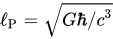
In 1972, Jacob Bekenstein conjectured that black holes should have an entropy proportional to the area of the event horizon, where by the same year, he proposed the no-hair theorem. In 1973 Bekenstein heuristically suggested ${\displaystyle \frac{\ln 2}{8\pi }\approx 0.0276}$ as the constant of proportionality. The next year, in 1974, Stephen Hawking showed that black holes emit thermal Hawking radiation corresponding to a certain temperature (Hawking temperature). Using the thermodynamic relationship between energy, temperature and entropy, Hawking was able to confirm Bekenstein's conjecture and fix the constant of proportionality at ${\displaystyle 1/4}$:

$${\displaystyle S_{\text{BH}}=\frac{k_{\text{B}}A}{4{{\ell }_{\text{P}}}^2},}$$

where ${\displaystyle A}$ is the area of the event horizon, ${\displaystyle k_{\text{B}}}$ is the Boltzmann constant, and ${\displaystyle {\ell }_{\text{P}}=\sqrt{G\hslash /c^3}}$ is the Planck length.

This is often referred to as the Bekenstein–Hawking formula. The subscript BH either stands for black hole or Bekenstein–Hawking. The fact that the black hole entropy is also the maximal entropy that can be obtained by the Bekenstein bound (wherein the Bekenstein bound becomes an equality) was the main observation that led to the holographic principle. This area relationship was generalized to arbitrary regions via the Ryu–Takayanagi formula, which relates the entanglement entropy of a boundary conformal field theory to a specific surface in its dual gravitational theory.

In the early 1990s Gerard 't Hooft and Leonard Susskind generalized the relationship between a black hole's surface area and its entropy, applying to all of spacetime. This was an early form of the holographic principle, a universal relationship between geometry and information. The idea is that the area surrounding any volume in spacetime limits the information content of the volume. Thus the number of degrees of freedom in any volume is bounded and not infinite.

Although Hawking's calculations gave further thermodynamic evidence for black hole entropy, until 1995 no one was able to make a controlled calculation of black hole entropy based on statistical mechanics, which associates entropy with a large number of microstates. Some work, called no-hair theorems, suggested that black holes could have only a single microstate. The situation changed in 1995 when Andrew Strominger and Cumrun Vafa calculated the Bekenstein–Hawking entropy of a supersymmetric black hole in string theory, using methods based on D-branes and string duality. Their calculation was followed by many similar computations of entropy of large classes of other extremal and near-extremal black holes, and the result always agreed with the Bekenstein–Hawking formula. However, for the Schwarzschild black hole, viewed as the furthest-from-extremal black hole, the relationship between micro- and macrostates has not been characterized. Efforts to develop an adequate answer within the framework of string theory continue.

In loop quantum gravity (LQG) it is possible to associate a geometrical interpretation with the microstates: these are the quantum geometries of the horizon. LQG offers a geometric explanation of the finiteness of the entropy and of the proportionality of the area of the horizon. It is possible to derive, from the covariant formulation of full quantum theory (spin foam), the correct relation between energy and area (first law), the Unruh temperature and the distribution that yields Hawking entropy. The calculation makes use of the notion of dynamical horizon and is done for non-extremal black holes. There seems to be also discussed the calculation of Bekenstein–Hawking entropy from the point of view of LQG. The current accepted microstate ensemble for black holes is the microcanonical ensemble. The partition function for black holes results in a negative heat capacity. In canonical ensembles, there is limitation for a positive heat capacity, whereas microcanonical ensembles can exist at a negative heat capacity.

Analyses of gravitational waves emitted by GW250114 confirmed Hawking's assertion that the surface area of a black hole is a non-decreasing function of time.

Laws of classical black hole mechanics

These four laws of black hole mechanics are relationships between physical properties of black holes assuming general relativity but no quantum effects. This form is analogous to the laws of thermodynamics but without quantum effects the black hole temperature must be zero and simply absorbs all radiation. This is the form proposed by Bardeen, Brandon Carter, and Hawking in 1973 (expressed in geometrized units).

Zeroth law

For a stationary black hole (one in mechanical equilibrium) the surface gravity, ${\displaystyle \kappa }$, is constant on the event horizon. This is the analog of the zeroth law of thermodynamics on the equivalence of temperature across a system at equilibrium with surface gravity being analogous to temperature.

First law

For perturbations of stationary black holes, the change of energy is related to change of area, angular momentum, and electric charge by

$${\displaystyle dE=\frac{\kappa }{8\pi }dA+\mathrm{\Omega }dJ+\mathrm{\Phi }dQ,}$$

where ${\displaystyle E}$ is the energy, ${\displaystyle \kappa }$ is the surface gravity, ${\displaystyle A}$ is the horizon area, ${\displaystyle \mathrm{\Omega }}$ is the angular velocity, ${\displaystyle J}$ is the angular momentum, ${\displaystyle \mathrm{\Phi }}$ is the electrostatic potential and ${\displaystyle Q}$ is the electric charge. Analogously, the first law of thermodynamics is a statement of energy conservation, which contains on its right side a term equal to temperature times change in entropy, ${\displaystyle TdS}$.

Second law

The horizon area is, assuming the weak energy condition, a non-decreasing function of time:

$${\displaystyle \frac{dA}{dt}\ge 0.}$$ Here black hole surface area is analogous to thermodynamic entropy and the laws say these properties can never spontaneously decrease.

Third law

It is not possible to form a black hole with vanishing surface gravity. That is, ${\displaystyle \kappa =0}$ cannot be achieved. This is analogous to some but not all forms of the third law of thermodynamics.

Quantum effects

The generalized second law of thermodynamics (GSL) is needed to present the second law of thermodynamics as valid. This is because the second law of thermodynamics, as a result of the disappearance of entropy near the exterior of black holes, is not useful. The GSL allows for the application of the law because it allows for the measurement of interior, common entropy. The validity of the GSL can be established by studying an example, such as looking at a system having entropy that falls into a bigger, non-moving black hole, and establishing upper and lower entropy bounds for the increase in the black hole entropy and entropy of the system, respectively. The GSL also holds for theories of gravity such as general relativity, Lovelock gravity, or braneworld gravity, because the conditions to use it for these theories can be met.

However, on the topic of black hole formation, the question becomes whether or not the generalized second law of thermodynamics will be valid, and if it is, it will have been proved valid for all situations. Because black hole formation is not a stationary event, proving that the GSL holds is difficult. Proving it is generally valid would require quantum-statistical mechanics, because the GSL is both a quantum and statistical law. This discipline does not exist so the GSL can be assumed to be useful in general, as well as for prediction. For example, one can use the GSL to predict that, for a cold, non-rotating assembly of ${\displaystyle N}$ nucleons, ${\displaystyle S_{\text{BH}}-S>0}$, where ${\displaystyle S_{\text{BH}}}$ is the entropy of a black hole and ${\displaystyle S}$ is the sum of the ordinary entropy.

Third law

The third law of black hole thermodynamics is controversial. Specific counterexamples called extremal black holes fail to obey the rule. The classical third law of thermodynamics, or Nernst's theorem, which says the entropy of a system must go to zero as the temperature goes to absolute zero, is also not a universal law. However, systems that fail the classical third law have not been realized in practice, leading to the suggestion that the extremal black holes may not represent the physics of black holes generally.

A weaker form of the classical third law known as the unattainability principle states that an infinite number of steps are required to put a system into its ground state. This form of the third law does have an analog in black hole physics.

Interpretation of the laws

The four laws of black hole mechanics suggest that one should identify the surface gravity of a black hole with temperature and the area of the event horizon with entropy, at least up to some multiplicative constants. If black holes are only considered classically, then they have zero temperature, and by the no-hair theorem, zero entropy, and the laws of black hole mechanics remain an analogy. However, when quantum-mechanical effects are taken into account, it is found that black holes emit thermal radiation (Hawking radiation) at the Hawking temperature.

$${\displaystyle T_{\text{H}}=\frac{\kappa }{2\pi }.}$$

From the first law of black hole mechanics, this determines the multiplicative constant of the Bekenstein–Hawking entropy, which is (in geometrized units)

$${\displaystyle S_{\text{BH}}=\frac{A}{4}.}$$

which is the entropy of the black hole in Einstein's general relativity. Quantum field theory in curved spacetime can be utilized to calculate the entropy for a black hole in any covariant theory for gravity, known as the Wald entropy.

Critique

While black hole thermodynamics (BHT) has been regarded as one of the deepest clues to a quantum theory of gravity, there remains criticism that "the analogy is not nearly as good as is commonly supposed", that it "is often based on a kind of caricature of thermodynamics" and "it's unclear what the systems in BHT are supposed to be".

Others have come to the opposite conclusion believing, "stationary black holes are not analogous to thermodynamic systems: they are thermodynamic systems, in the fullest sense."

Diffuse sky radiation

From Wikipedia, the free encyclopedia

https://en.wikipedia.org/wiki/Diffuse_sky_radiation

In Earth's atmosphere, the dominant scattering efficiency of blue light is compared to red or green light. Scattering and absorption are major causes of the attenuation of sunlight radiation by the atmosphere. During broad daylight, the sky is blue due to Rayleigh scattering, while around sunrise or sunset, and especially during twilight, absorption of irradiation by ozone helps maintain blue color in the evening sky. At sunrise or sunset, tangentially incident solar rays illuminate clouds with orange to red hues.

The visible spectrum, approximately 380 to 740 nanometers (nm),^[1] shows the atmospheric water absorption band and the solar Fraunhofer lines. The blue sky spectrum contains light at all visible wavelengths with a broad maximum around 450–485 nm, the wavelengths of the color blue.

Diffuse sky radiation, is solar radiation reaching the Earth's surface after having been scattered from the direct solar beam by molecules or particulates in the atmosphere. It is also called sky radiation, the determinative process for changing the colors of the sky. It is normally measured on a horizontal surface, thus frequently termed diffuse horizontal irradiance (DHI), often in the unit of watts per square meter (W/m²). Approximately 23% of direct incident radiation of total sunlight is removed from the direct solar beam by scattering into the atmosphere; of this amount (of incident radiation) about two-thirds ultimately reaches the earth as photon diffused skylight radiation.

The dominant radiative scattering processes in the atmosphere are Rayleigh scattering and Mie scattering; they are elastic, meaning that a photon of light can be deviated from its path without being absorbed and without changing wavelength.

Under an overcast sky, there is no direct sunlight, and all light results from diffused skylight radiation.

Proceeding from analyses of the aftermath of the eruption of the Philippines volcano Mount Pinatubo (in June 1991) and other studies: Diffused skylight, owing to its intrinsic structure and behavior, can illuminate under-canopy leaves, permitting more efficient total whole-plant photosynthesis than would otherwise be the case; this in stark contrast to the effect of totally clear skies with direct sunlight that casts shadows onto understory leaves and thereby limits plant photosynthesis to the top canopy layer, (see below).

Color

A clear daytime sky, looking toward the zenith

Earth's atmosphere scatters short-wavelength light more efficiently than that of longer wavelengths. Because its wavelengths are shorter, blue light is more strongly scattered than the longer-wavelength lights, red or green. Hence, the result that when looking at the sky away from the direct incident sunlight, the human perceives the sky to be blue. The color perceived is similar to that presented by a monochromatic blue (at wavelength 474–476 nm) mixed with white light, that is, an unsaturated blue light. The explanation of blue color by Lord Rayleigh in 1871 is a famous example of applying dimensional analysis to solving problems in physics.

Scattering and absorption are major causes of the attenuation of sunlight radiation by the atmosphere. Scattering varies as a function of the ratio of particle diameters (of particulates in the atmosphere) to the wavelength of the incident radiation. When this ratio is less than about one-tenth, Rayleigh scattering occurs. (In this case, the scattering coefficient varies inversely with the fourth power of the wavelength. At larger ratios scattering varies in a more complex fashion, as described for spherical particles by the Mie theory.) The laws of geometric optics begin to apply at higher ratios.

Daily at any global venue experiencing sunrise or sunset, most of the solar beam of visible sunlight arrives nearly tangentially to Earth's surface. Here, the path of sunlight through the atmosphere is elongated such that much of the blue or green light is scattered away from the line of perceivable visible light. This phenomenon leaves the Sun's rays, and the clouds they illuminate, abundantly orange-to-red in colors, which one sees when looking at a sunset or sunrise.

For the example of the Sun at zenith, in broad daylight, the sky is blue due to Rayleigh scattering, which also involves the diatomic gases N
₂ and O
₂. Near sunset and especially during twilight, absorption by ozone (O
₃) significantly contributes to maintaining blue color in the evening sky.

Under an overcast sky

There is essentially no direct sunlight under an overcast sky, so all light is then diffuse sky radiation. The flux of light is not very wavelength-dependent because the cloud droplets are larger than the light's wavelength and scatter all colors approximately equally. The light passes through the translucent clouds in a manner similar to frosted glass. The intensity ranges (roughly) from 1⁄6 of direct sunlight for relatively thin clouds down to 1⁄1000 of direct sunlight under the extreme of thickest storm clouds.

As a part of total radiation on a horizontal surface

The diffuse horizontal irradiance is part of the global horizontal irradiance and the following relation holds for instantaneous measurements $${\displaystyle \text{GHI}=\text{DHI}+\text{DNI}\times \cos (z)=\text{DHI}+\text{DirHI}}$$ where GHI is the global horizontal irradiance, DHI is the diffuse horizontal irradiance, DNI is the direct normal irradiance, ${\displaystyle z}$ is the solar zenith angle, and DirHI is the direct horizontal irradiance.

As a part of total radiation on a southward tilted surface

One of the equations for total solar radiation on a southward tilted surface is:

${\displaystyle H_t=H_b{R}_b+H_d{R}_d+(H_b+H_d)R_r}$

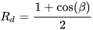
where H_b is the beam radiation irradiance, R_b is the tilt factor for beam radiation, H_d is the diffuse radiation irradiance, R_d is the tilt factor for diffuse radiation and R_r is the tilt factor for reflected radiation.

R_b is given by:

${\displaystyle R_b=\frac{\sin (\delta )\sin (\varphi -\beta )+\cos (\delta )\cos (h)\cos (\varphi -\beta )}{\sin (\delta )\sin (\varphi )+\cos (\delta )\cos (h)\cos (\varphi )}}$

where δ is the solar declination, Φ is the latitude, β is an angle from the horizontal and h is the solar hour angle.

R_d is given by:

${\displaystyle R_d=\frac{1+\cos (\beta )}{2}}$

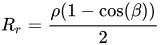
and R_r by:

${\displaystyle R_r=\frac{\rho (1-\cos (\beta ))}{2}}$

where ρ is the reflectivity of the surface.

Agriculture and the eruption of Mt. Pinatubo

A Space Shuttle (Mission STS-43) photograph of the Earth over South America taken on August 8, 1991, which captures the double layer of Pinatubo aerosol clouds (dark streaks) above lower cloud tops

The eruption of the Philippines volcano - Mount Pinatubo in June 1991 ejected roughly 10 km³ (2.4 cu mi) of magma and "17 million metric tons"(17 teragrams) of sulfur dioxide SO₂ into the air, introducing ten times as much total SO₂ as the 1991 Kuwaiti fires,^[8] mostly during the explosive Plinian/Ultra-Plinian event of June 15, 1991, creating a global stratospheric SO₂ haze layer which persisted for years. This resulted in the global average temperature dropping by about 0.5 °C (0.9 °F). Since volcanic ash falls out of the atmosphere rapidly, the negative agricultural, effects of the eruption were largely immediate and localized to a relatively small area in close proximity to the eruption, caused by the resulting thick ash cover. Globally however, despite a several-month 5% drop in overall solar irradiation, and a reduction in direct sunlight by 30%, there was no negative impact on global agriculture. Surprisingly, a 3-4 year increase in global Agricultural productivity and forestry growth was observed, excepting boreal forest regions.

Under more-or-less direct sunlight, dark shadows that limit photosynthesis are cast onto understorey leaves. Within the thicket, very little direct sunlight can enter.

The means of discovery was that initially, a mysterious drop in the rate at which carbon dioxide (CO₂) was filling the atmosphere was observed, which is charted in what is known as the "Keeling Curve". This led numerous scientists to assume that the reduction was due to the lowering of Earth's temperature, and with that, a, slowdown in plant and soil respiration, indicating a deleterious impact on global agriculture from the volcanic haze layer. However upon investigation, the reduction in the rate at which carbon dioxide filled the atmosphere did not match up with the hypothesis that plant respiration rates had declined. Instead the advantageous anomaly was relatively firmly linked to an unprecedented increase in the growth/net primary production, of global plant life, resulting in the increase of the carbon sink effect of global photosynthesis. The mechanism by which the increase in plant growth was possible, was that the 30% reduction of direct sunlight can also be expressed as an increase or "enhancement" in the amount of diffuse sunlight.

The diffused skylight effect

Well lit understorey areas due to overcast clouds creating diffuse/soft sunlight conditions, that permits photosynthesis on leaves under the canopy.

This diffused skylight, owing to its intrinsic nature, can illuminate under-canopy leaves permitting more efficient total whole-plant photosynthesis than would otherwise be the case, and also increasing evaporative cooling, from vegetated surfaces. In stark contrast, for totally clear skies and the direct sunlight that results from it, shadows are cast onto understorey leaves, limiting plant photosynthesis to the top canopy layer. This increase in global agriculture from the volcanic haze layer also naturally results as a product of other aerosols that are not emitted by volcanoes, such, "moderately thick smoke loading" pollution, as the same mechanism, the "aerosol direct radiative effect" is behind both.

Probability density function

From Wikipedia, the free encyclopedia

https://en.wikipedia.org/wiki/Probability_density_function 

Box plot and probability density function of a normal distribution N(0, σ²).

Geometric visualisation of the mode, median and mean of an arbitrary unimodal probability density function.

In probability theory, a probability density function (PDF), density function, or simply density of an absolutely continuous random variable, is a function whose value at any given point in the sample space (the set of possible values taken by the random variable) can be interpreted as providing a "relative probability" that the value of the random variable would be equal to that point. Probability density is the probability per unit length, in other words. The (absolute) probability for a continuous random variable to take on any particular value is zero. Therefore, the value of the PDF at two different samples can be used to infer, in any particular draw of the random variable, how much more likely it is that the random variable would be close to one point compared to the other.

More precisely, the PDF is used to specify the probability of the random variable falling within a particular range of values, as opposed to taking on any one value. This probability is given by the integral of a continuous variable's PDF over that range, where the integral is the nonnegative area under the density function between the lowest and greatest values of the range. The PDF is nonnegative everywhere, and the area under the entire curve is equal to one, such that the probability of the random variable falling within the set of possible values is 100%.

The terms probability distribution function and probability function can also denote the probability density function. However, this use is not standard among probabilists and statisticians. In other sources, "probability distribution function" may be used when the probability distribution is defined as a function over general sets of values or it may refer to the cumulative distribution function (CDF), or it may be a probability mass function (PMF) rather than the density. Density function itself is also used for the probability mass function, leading to further confusion. In general the PMF is used in the context of discrete random variables (random variables that take values on a countable set), while the PDF is used in the context of continuous random variables. Both PMF and PDF are fundamental concepts in statistical inference.

Example

Examples of four continuous probability density functions.

Suppose bacteria of a certain species typically live 20 to 30 hours. The probability that a bacterium lives exactly 5 hours is equal to zero (we are talking about an idealized real-valued variable, not the recorded observation). A lot of bacteria live for approximately 5 hours, but there is no chance that any given bacterium dies at exactly 5.00... hours (measured with infinite precision). However, the probability that the bacterium dies between 5 hours and 5.01 hours is quantifiable. Suppose the answer is 0.02 (i.e., 2%). Then, the probability that the bacterium dies between 5 hours and 5.001 hours should be about 0.002, since this time interval is one-tenth as long as the previous. The probability that the bacterium dies between 5 hours and 5.0001 hours should be about 0.0002, and so on.

In this example, the ratio (probability of dying during an interval) / (duration of the interval) is approximately constant, and equal to 2 per hour (or 2 hour⁻¹). For example, there is 0.02 probability of dying in the 0.01-hour interval between 5 and 5.01 hours, and (0.02 probability / 0.01 hours) = 2 hour⁻¹. This quantity 2 hour⁻¹ is called the probability density for dying at around 5 hours. Therefore, the probability that the bacterium dies at 5 hours can be written as (2 hour⁻¹) dt. This is the probability that the bacterium dies within an infinitesimal window of time around 5 hours, where dt is the duration of this window. For example, the probability that it lives longer than 5 hours, but shorter than (5 hours + 1 nanosecond), is (2 hour⁻¹)×(1 nanosecond) ≈ 6×10⁻¹³ (using the unit conversion 3.6×10¹² nanoseconds = 1 hour).

There is a probability density function f with f(5 hours) = 2 hour⁻¹. The integral of f over any window of time (not only infinitesimal windows but also large windows) is the probability that the bacterium dies in that window.

Absolutely continuous univariate distributions

A probability density function is most commonly associated with absolutely continuous univariate distributions. A random variable ${\displaystyle X}$ has density ${\displaystyle f_X}$, where ${\displaystyle f_X}$ is a non-negative Lebesgue-integrable function, if: $${\displaystyle Pr[a\le X\le b]={\int }_a^b{f}_X(x)dx.}$$

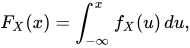
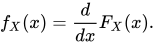
Hence, if ${\displaystyle F_X}$ is the cumulative distribution function of ${\displaystyle X}$, then: $${\displaystyle F_X(x)={\int }_{-\mathrm{\infty }}^x{f}_X(u)du,}$$ and (if ${\displaystyle F_X}$ is differentiable at ${\displaystyle x}$) $${\displaystyle f_X(x)=\frac{d}{dx}{F}_X(x).}$$

Intuitively, one can think of ${\displaystyle f_X(x)dx}$ as being the probability of ${\displaystyle X}$ falling within the infinitesimal interval ${\displaystyle [x,x+dx]}$.

Formal definition

(This definition may be extended to any probability distribution using the measure-theoretic definition of probability.)

A random variable ${\displaystyle X}$ with values in a measurable space ${\displaystyle (\mathcal{X},\mathcal{A})}$ (usually ${\displaystyle {\mathbb{R}}^n}$ with the Borel sets as measurable subsets) has as probability distribution the pushforward measure X_∗P on ${\displaystyle (\mathcal{X},\mathcal{A})}$: the density of ${\displaystyle X}$ with respect to a reference measure ${\displaystyle \mu }$ on ${\displaystyle (\mathcal{X},\mathcal{A})}$ is the Radon–Nikodym derivative: $${\displaystyle f=\frac{d{X}_{\ast }P}{d\mu }.}$$

That is, f is any measurable function with the property that: $${\displaystyle Pr[X\in A]={\int }_{X^{-1}A}dP={\int }_{A}fd\mu }$$ for any measurable set ${\displaystyle A\in \mathcal{A}.}$

Discussion

In the continuous univariate case above, the reference measure is the Lebesgue measure. The probability mass function of a discrete random variable is the density with respect to the counting measure over the sample space (usually the set of integers, or some subset thereof).

It is not possible to define a density with reference to an arbitrary measure (e.g. one can not choose the counting measure as a reference for a continuous random variable). Furthermore, when it does exist, the density is almost unique, meaning that any two such densities coincide almost everywhere.

Further details

Unlike a probability, a probability density function can take on values greater than one; for example, the continuous uniform distribution on the interval [0, 1/2] has probability density f(x) = 2 for 0 ≤ x ≤ 1/2 and f(x) = 0 elsewhere.

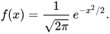
The standard normal distribution has probability density$${\displaystyle f(x)=\frac{1}{\sqrt{2\pi }}{e}^{-x^2/2}.}$$

If a random variable X is given and its distribution admits a probability density function f, then the expected value of X (if the expected value exists) can be calculated as$${\displaystyle \mathrm{E}[X]={\int }_{-\mathrm{\infty }}^{\mathrm{\infty }}xf(x)dx.}$$

Not every probability distribution has a density function: the distributions of discrete random variables do not; nor does the Cantor distribution, even though it has no discrete component, i.e., does not assign positive probability to any individual point.

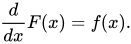
A distribution has a density function if its cumulative distribution function F(x) is absolutely continuous. In this case: F is almost everywhere differentiable, and its derivative can be used as probability density:$${\displaystyle \frac{d}{dx}F(x)=f(x).}$$

If a probability distribution admits a density, then the probability of every one-point set {a} is zero; the same holds for finite and countable sets.

Two probability densities f and g represent the same probability distribution precisely if they differ only on a set of Lebesgue measure zero.

In the field of statistical physics, a non-formal reformulation of the relation above between the derivative of the cumulative distribution function and the probability density function is generally used as the definition of the probability density function. This alternate definition is the following:

If dt is an infinitely small number, the probability that X is included within the interval (t, t + dt) is equal to f(t) dt, or: $${\displaystyle Pr(t<X<t+dt)=f(t)dt.}$$

Link between discrete and continuous distributions

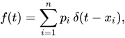
It is possible to represent certain discrete random variables as well as random variables involving both a continuous and a discrete part with a generalized probability density function using the Dirac delta function. (This is not possible with a probability density function in the sense defined above, it may be done with a distribution.) For example, consider a binary discrete random variable having the Rademacher distribution—that is, taking −1 or 1 for values, with probability 1⁄2 each. The density of probability associated with this variable is: $${\displaystyle f(t)=\frac{1}{2}(\delta (t+1)+\delta (t-1)).}$$

More generally, if a discrete variable can take n different values among real numbers, then the associated probability density function is: $${\displaystyle f(t)=\sum _{i=1}^n{p}_i\delta (t-x_i),}$$ where ${\displaystyle x_1,\dots ,x_n}$ are the discrete values accessible to the variable and ${\displaystyle p_1,\dots ,p_n}$ are the probabilities associated with these values.

This substantially unifies the treatment of discrete and continuous probability distributions. The above expression allows for determining statistical characteristics of such a discrete variable (such as the mean, variance, and kurtosis), starting from the formulas given for a continuous distribution of the probability.

Families of densities

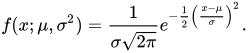
It is common for probability density functions (and probability mass functions) to be parametrized—that is, to be characterized by unspecified parameters. For example, the normal distribution is parametrized in terms of the mean and the variance, denoted by ${\displaystyle \mu }$ and ${\displaystyle {\sigma }^2}$ respectively, giving the family of densities $${\displaystyle f(x;\mu ,{\sigma }^2)=\frac{1}{\sigma \sqrt{2\pi }}{e}^{-\frac{1}{2}{\left(\frac{x-\mu }{\sigma }\right)}^2}.}$$ Different values of the parameters describe different distributions of different random variables on the same sample space (the same set of all possible values of the variable); this sample space is the domain of the family of random variables that this family of distributions describes. A given set of parameters describes a single distribution within the family sharing the functional form of the density. From the perspective of a given distribution, the parameters are constants, and terms in a density function that contain only parameters, but not variables, are part of the normalization factor of a distribution (the multiplicative factor that ensures that the area under the density—the probability of something in the domain occurring— equals 1). This normalization factor is outside the kernel of the distribution.

Since the parameters are constants, reparametrizing a density in terms of different parameters to give a characterization of a different random variable in the family, means simply substituting the new parameter values into the formula in place of the old ones.

Densities associated with multiple variables

For continuous random variables X₁, ..., X_n, it is also possible to define a probability density function associated to the set as a whole, often called joint probability density function. This density function is defined as a function of the n variables, such that, for any domain D in the n-dimensional space of the values of the variables X₁, ..., X_n, the probability that a realisation of the set variables falls inside the domain D is $${\displaystyle Pr\left(X_1,\dots ,X_n\in D\right)={\int }_D{f}_{X_1,\dots ,X_n}(x_1,\dots ,x_n)d{x}_1\cdots d{x}_n.}$$

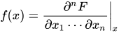
If F(x₁, ..., x_n) = Pr(X₁ ≤ x₁, ..., X_n ≤ x_n) is the cumulative distribution function of the vector (X₁, ..., X_n), then the joint probability density function can be computed as a partial derivative $${\displaystyle f(x)={\frac{{\mathrm{\partial }}^{n}F}{\mathrm{\partial }{x}_1\cdots \mathrm{\partial }{x}_n}|}_x}$$

Marginal densities

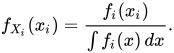
For i = 1, 2, ..., n, let f_Xi(x_i) be the probability density function associated with variable X_i alone. This is called the marginal density function, and can be deduced from the probability density associated with the random variables X₁, ..., X_n by integrating over all values of the other n − 1 variables: $${\displaystyle f_{X_i}(x_i)=\int f(x_1,\dots ,x_n)d{x}_1\cdots d{x}_{i-1}d{x}_{i+1}\cdots d{x}_n.}$$

Independence

Continuous random variables X₁, ..., X_n admitting a joint density are all independent from each other if $${\displaystyle f_{X_1,\dots ,X_n}(x_1,\dots ,x_n)=f_{X_1}(x_1)\cdots f_{X_n}(x_n).}$$

Corollary

If the joint probability density function of a vector of n random variables can be factored into a product of n functions of one variable $${\displaystyle f_{X_1,\dots ,X_n}(x_1,\dots ,x_n)=f_1(x_1)\cdots f_n(x_n),}$$ (where each f_i is not necessarily a density) then the n variables in the set are all independent from each other, and the marginal probability density function of each of them is given by $${\displaystyle f_{X_i}(x_i)=\frac{f_i(x_i)}{\int f_i(x)dx}.}$$

Example

This elementary example illustrates the above definition of multidimensional probability density functions in the simple case of a function of a set of two variables. Let us call ${\displaystyle \overrightarrow{R}}$ a 2-dimensional random vector of coordinates (X, Y): the probability to obtain ${\displaystyle \overrightarrow{R}}$ in the quarter plane of positive x and y is $${\displaystyle Pr\left(X>0,Y>0\right)={\int }_0^{\mathrm{\infty }}{\int }_0^{\mathrm{\infty }}{f}_{X,Y}(x,y)dxdy.}$$

Function of random variables and change of variables in the probability density function

If the probability density function of a random variable (or vector) X is given as f_X(x), it is possible (but often not necessary; see below) to calculate the probability density function of some variable Y = g(X). This is also called a "change of variable" and is in practice used to generate a random variable of arbitrary shape f_g(X) = f_Y using a known (for instance, uniform) random number generator.

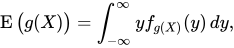
It is tempting to think that in order to find the expected value E(g(X)), one must first find the probability density f_g(X) of the new random variable Y = g(X). However, rather than computing $${\displaystyle \mathrm{E}(g(X))={\int }_{-\mathrm{\infty }}^{\mathrm{\infty }}y{f}_{g(X)}(y)dy,}$$ one may find instead $${\displaystyle \mathrm{E}(g(X))={\int }_{-\mathrm{\infty }}^{\mathrm{\infty }}g(x)f_X(x)dx.}$$

The values of the two integrals are the same in all cases in which both X and g(X) actually have probability density functions. It is not necessary that g be a one-to-one function. In some cases the latter integral is computed much more easily than the former. See Law of the unconscious statistician.

Scalar to scalar

Let ${\displaystyle g:\mathbb{R}\to \mathbb{R}}$ be a monotonic function, then the resulting density function is $${\displaystyle f_Y(y)=f_X(g^{-1}(y))\left|\frac{d}{dy}(g^{-1}(y))\right|.}$$

Here g⁻¹ denotes the inverse function.

This follows from the fact that the probability contained in a differential area must be invariant under change of variables. That is, $${\displaystyle \left|f_Y(y)dy\right|=\left|f_X(x)dx\right|,}$$ or $${\displaystyle f_Y(y)=\left|\frac{dx}{dy}\right|f_X(x)=\left|\frac{d}{dy}(x)\right|f_X(x)=\left|\frac{d}{dy}(g^{-1}(y))\right|f_X(g^{-1}(y))=\left|{\left(g^{-1}\right)}^{\prime }(y)\right|\cdot f_X(g^{-1}(y)).}$$

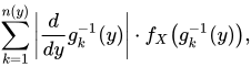
For functions that are not monotonic, the probability density function for y is $${\displaystyle \sum _{k=1}^{n(y)}\left|\frac{d}{dy}{g}_k^{-1}(y)\right|\cdot f_X(g_k^{-1}(y)),}$$ where n(y) is the number of solutions in x for the equation ${\displaystyle g(x)=y}$, and ${\displaystyle g_k^{-1}(y)}$ are these solutions.

Vector to vector

Suppose x is an n-dimensional random variable with joint density f. If y = G(x), where G is a bijective, differentiable function, then y has density p_Y: $${\displaystyle p_Y(\mathbf{y})=f(G^{-1}(\mathbf{y}))\left|det\left[{\frac{d{G}^{-1}(\mathbf{z})}{d\mathbf{z}}|}_{\mathbf{z}=\mathbf{y}}\right]\right|}$$ with the differential regarded as the Jacobian of the inverse of G(⋅), evaluated at y.

For example, in the 2-dimensional case x = (x₁, x₂), suppose the transform G is given as y₁ = G₁(x₁, x₂), y₂ = G₂(x₁, x₂) with inverses x₁ = G₁⁻¹(y₁, y₂), x₂ = G₂⁻¹(y₁, y₂). The joint distribution for y = (y₁, y₂) has density $${\displaystyle p_{Y_1,Y_2}(y_1,y_2)=f_{X_1,X_2}(G_1^{-1}(y_1,y_2),G_2^{-1}(y_1,y_2))\left|\frac{\mathrm{\partial }{G}_1^{-1}}{\mathrm{\partial }{y}_1}\frac{\mathrm{\partial }{G}_2^{-1}}{\mathrm{\partial }{y}_2}-\frac{\mathrm{\partial }{G}_1^{-1}}{\mathrm{\partial }{y}_2}\frac{\mathrm{\partial }{G}_2^{-1}}{\mathrm{\partial }{y}_1}\right|.}$$

Vector to scalar

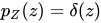
Let ${\displaystyle V:{\mathbb{R}}^n\to \mathbb{R}}$ be a differentiable function and ${\displaystyle X}$ be a random vector taking values in ${\displaystyle {\mathbb{R}}^n}$, ${\displaystyle f_X}$ be the probability density function of ${\displaystyle X}$ and ${\displaystyle \delta (\cdot )}$ be the Dirac delta function. It is possible to use the formulas above to determine ${\displaystyle f_Y}$, the probability density function of ${\displaystyle Y=V(X)}$, which will be given by $${\displaystyle f_Y(y)={\int }_{{\mathbb{R}}^n}{f}_X(\mathbf{x})\delta (y-V(\mathbf{x}))d\mathbf{x}.}$$

This result leads to the law of the unconscious statistician: $${\displaystyle \begin{array}{rl}{\mathrm{E}}_Y[Y]& ={\int }_{\mathbb{R}}y{f}_Y(y)dy\\ & ={\int }_{\mathbb{R}}y{\int }_{{\mathbb{R}}^n}{f}_X(\mathbf{x})\delta (y-V(\mathbf{x}))d\mathbf{x}dy\\ & ={\int }_{{\mathbb{R}}^n}{\int }_{\mathbb{R}}y{f}_X(\mathbf{x})\delta (y-V(\mathbf{x}))dyd\mathbf{x}\\ & ={\int }_{{\mathbb{R}}^n}V(\mathbf{x})f_X(\mathbf{x})d\mathbf{x}={\mathrm{E}}_X[V(X)].\end{array}}$$

Proof:

Let ${\displaystyle Z}$ be a collapsed random variable with probability density function ${\displaystyle p_Z(z)=\delta (z)}$ (i.e., a constant equal to zero). Let the random vector ${\displaystyle \tilde{X}}$ and the transform ${\displaystyle H}$ be defined as $${\displaystyle H(Z,X)=\left[\begin{array}{c}Z+V(X)\\ X\end{array}\right]=\left[\begin{array}{c}Y\\ \tilde{X}\end{array}\right].}$$

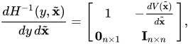
It is clear that ${\displaystyle H}$ is a bijective mapping, and the Jacobian of ${\displaystyle H^{-1}}$ is given by: $${\displaystyle \frac{d{H}^{-1}(y,\tilde{\mathbf{x}})}{dyd\tilde{\mathbf{x}}}=\left[\begin{array}{cc}1& -\frac{dV(\tilde{\mathbf{x}})}{d\tilde{\mathbf{x}}}\\ {\mathbf{0}}_{n\times 1}& {\mathbf{I}}_{n\times n}\end{array}\right],}$$ which is an upper triangular matrix with ones on the main diagonal, therefore its determinant is 1. Applying the change of variable theorem from the previous section we obtain that $${\displaystyle f_{Y,X}(y,x)=f_X(\mathbf{x})\delta (y-V(\mathbf{x})),}$$ which if marginalized over ${\displaystyle x}$ leads to the desired probability density function.

Sums of independent random variables

See also: List of convolutions of probability distributions

The probability density function of the sum of two independent random variables U and V, each of which has a probability density function, is the convolution of their separate density functions: $${\displaystyle f_{U+V}(x)={\int }_{-\mathrm{\infty }}^{\mathrm{\infty }}{f}_U(y)f_V(x-y)dy=\left(f_U\ast f_V\right)(x)}$$

It is possible to generalize the previous relation to a sum of N independent random variables, with densities U₁, ..., U_N: $${\displaystyle f_{U_1+\cdots +U}(x)=\left(f_{U_1}\ast \cdots \ast f_{U_N}\right)(x)}$$

This can be derived from a two-way change of variables involving Y = U + V and Z = V, similarly to the example below for the quotient of independent random variables.

Products and quotients of independent random variables

See also: Product distribution and Ratio distribution

Given two independent random variables U and V, each of which has a probability density function, the density of the product Y = UV and quotient Y = U/V can be computed by a change of variables.

Example: Quotient distribution

To compute the quotient Y = U/V of two independent random variables U and V, define the following transformation: $${\displaystyle \begin{array}{rl}Y& =U/V\\ Z& =V\end{array}}$$

Then, the joint density p(y,z) can be computed by a change of variables from U,V to Y,Z, and Y can be derived by marginalizing out Z from the joint density.

The inverse transformation is $${\displaystyle \begin{array}{rl}U& =YZ\\ V& =Z\end{array}}$$

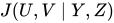
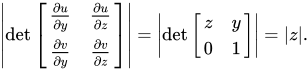
The absolute value of the Jacobian matrix determinant ${\displaystyle J(U,V\mid Y,Z)}$ of this transformation is: $${\displaystyle \left|det\left[\begin{array}{cc}\frac{\mathrm{\partial }u}{\mathrm{\partial }y}& \frac{\mathrm{\partial }u}{\mathrm{\partial }z}\\ \frac{\mathrm{\partial }v}{\mathrm{\partial }y}& \frac{\mathrm{\partial }v}{\mathrm{\partial }z}\end{array}\right]\right|=\left|det\left[\begin{array}{cc}z& y\\ 0& 1\end{array}\right]\right|=|z|.}$$

Thus: $${\displaystyle p(y,z)=p(u,v)J(u,v\mid y,z)=p(u)p(v)J(u,v\mid y,z)=p_U(yz)p_V(z)|z|.}$$

And the distribution of Y can be computed by marginalizing out Z: $${\displaystyle p(y)={\int }_{-\mathrm{\infty }}^{\mathrm{\infty }}{p}_U(yz)p_V(z)|z|dz}$$

This method crucially requires that the transformation from U,V to Y,Z be bijective. The above transformation meets this because Z can be mapped directly back to V, and for a given V the quotient U/V is monotonic. This is similarly the case for the sum U + V, difference U − V and product UV.

Exactly the same method can be used to compute the distribution of other functions of multiple independent random variables.

Example: Quotient of two standard normals

Given two standard normal variables U and V, the quotient can be computed as follows. First, the variables have the following density functions: $${\displaystyle \begin{array}{rl}p(u)& =\frac{1}{\sqrt{2\pi }}{e}^{-u^2/2}\\ p(v)& =\frac{1}{\sqrt{2\pi }}{e}^{-v^2/2}\end{array}}$$

We transform as described above: $${\displaystyle \begin{array}{rl}Y& =U/V\\ Z& =V\end{array}}$$

This leads to: $${\displaystyle \begin{array}{rl}p(y)& ={\int }_{-\mathrm{\infty }}^{\mathrm{\infty }}{p}_U(yz)p_V(z)|z|dz\\ & ={\int }_{-\mathrm{\infty }}^{\mathrm{\infty }}\frac{1}{\sqrt{2\pi }}{e}^{-\frac{1}{2}{y}^2{z}^2}\frac{1}{\sqrt{2\pi }}{e}^{-\frac{1}{2}{z}^2}|z|dz\\ & ={\int }_{-\mathrm{\infty }}^{\mathrm{\infty }}\frac{1}{2\pi }{e}^{-\frac{1}{2}\left(y^2+1\right)z^2}|z|dz\\ & =2{\int }_0^{\mathrm{\infty }}\frac{1}{2\pi }{e}^{-\frac{1}{2}\left(y^2+1\right)z^2}zdz\\ & ={\int }_0^{\mathrm{\infty }}\frac{1}{\pi }{e}^{-\left(y^2+1\right)u}du& & u=\frac{1}{2}{z}^2\\ & ={-\frac{1}{\pi \left(y^2+1\right)}{e}^{-\left(y^2+1\right)u}|}_{u=0}^{\mathrm{\infty }}\\ & =\frac{1}{\pi \left(y^2+1\right)}\end{array}}$$

This is the density of a standard Cauchy distribution.