Compatibilism is the belief that free will and determinism are mutually compatible and that it is possible to believe in both without being logically inconsistent. The opposing belief, that the thesis of determinism is logically incompatible with the classical thesis of free will, is known as "incompatibilism".
Compatibilists often believe that freedom can be present or absent in situations for reasons that have nothing to do with metaphysics. In other words, that causal determinism does not exclude the truth of possible future outcomes. Because free will is often seen as a necessary prerequisite for moral responsibility, compatibilism is commonly used to support compatibility between moral responsibility and determinism.
Similarly, political liberty is a non-metaphysical concept. Statements of political liberty, such as the United States Bill of Rights, assume moral liberty: the ability to choose to do otherwise than what one does.
History
Compatibilism was championed by the ancient Stoics and some medieval scholastics. More specifically, scholastics like Thomas Aquinas and later Thomists (such as Domingo Báñez)
are often interpreted as holding that human action can be free, even
though an agent in some strong sense could not do otherwise than what
they did. Whereas Aquinas is often interpreted to maintain rational
compatibilism (i.e., an action can be determined by rational cognition
and yet free), later Thomists, such as Báñez, develop a sophisticated
theory of theological determinism, according to which actions of free
agents, despite being free, are, on a higher level, determined by
infallible divine decrees manifested in the form of "physical premotion" (praemotio physica),
a deterministic intervention of God into the will of a free agent
required to reduce the will from potency to act. A strong
incompatibilist view of freedom was, on the other hand, developed in the
Franciscan tradition, especially by Duns Scotus, and later upheld and further developed by Jesuits, especially Luis de Molina and Francisco Suárez. In the early modern era, compatibilism was maintained by Age of Enlightenment philosophers such as David Hume and Thomas Hobbes.
During the 20th century, compatibilists presented novel
arguments that differed from the classical arguments of Hume, Hobbes,
and John Stuart Mill. Importantly, Harry Frankfurt popularized what are now known as Frankfurt counterexamples
to argue for semicompatibilism, the view that determinism is compatible
with moral responsibility regardless of its compatibility with free
will, and developed a positive account of semicompatibilism based on higher-order volitions. Other "new compatibilists" include Gary Watson, Susan R. Wolf, P. F. Strawson, Kadri Vihvelin, and R. Jay Wallace. Contemporary compatibilists range from the philosopher and cognitive scientist Daniel Dennett, particularly in his works Elbow Room (1984) and Freedom Evolves (2003), to the existentialist philosopher Frithjof Bergmann. Perhaps the most renowned contemporary defender of semicompatibilism is John Martin Fischer. Other semicompatibilists include David P. Hunt and Alfred Mele.
A 2020 survey found that 59% of English-publishing philosophers accept or lean towards compatibilism.
Compatibilists often define an instance of "free will" as one in which the agent had the freedom to act according to their own motivation. That is, the agent was not coerced or restrained. Arthur Schopenhauer famously said: "Man can do what he wills but he cannot will what he wills". In other words, although an agent may often be free to act according to a motive, the nature of that motive is determined. This definition of free will does not rely on the truth or falsity of causal determinism. This view also makes free will close to autonomy, the ability to live according to one's own rules, as opposed to being submitted to external domination.
Daniel Dennett expands on this idea in his book Elbow Room,
arguing that in seeking free will we must consider what exactly is
desired in the concept of free will. He argues that if one becomes
convinced of the need for some capacity, such as the ability to have done otherwise,
it is because we have become convinced that this capacity is necessary
"for the sort of free will that any responsible, dignified, moral agent
must have." Dennett then says the following regarding what is requested of free will:
What we want when
we want free will is the power to decide our courses of action, and to
decide them wisely, in light of our expectations and desires. We want to
be in control of ourselves, and not under the control of others.
(. . .)
We want, moreover, to have enough elbow room in the world so that when
we exercise these powers, it is not always a matter of settling for the
only desperate course of action that has a chance of fulfilling our
desires.
—Daniel Dennett, Elbow Room, p. 184
Dennett argues that determinism itself does not restrict us
from reaching or accomplishing any of that which we seek out of free
will, and so determinism is compatible with free will, or at least any
"free will worth wanting"
Alternatives as imaginary
Schrödinger's door: Saying "there may be a person behind that door" merely expresses ignorance about the one, determined reality.
Some compatibilists hold both causal determinism (all effects have causes) and logical determinism
(the future is already determined) to be true. Thus statements about
the future (e.g., "it will rain tomorrow") are either true or false when
spoken today. This compatibilist free will should not be understood as
the ability to choose differently in an identical situation. A
compatibilist may believe that a person can decide between several
choices, but the choice is always determined by external factors. If the compatibilist says "I may visit tomorrow, or I may not", he is
saying that he does not know what he will choose—whether he will choose
to follow the subconscious urge to go or not.
Alternatives to strictly naturalist physics, such as mind–body dualism
positing a mind or soul existing apart from one's body while
perceiving, thinking, choosing freely, and as a result acting
independently on the body, include both traditional religious
metaphysics and less common newer compatibilist concepts. Also consistent with both autonomy and Darwinism, they allow for free personal agency based on practical reasons within the laws of physics. While less popular among 21st-century philosophers, non-naturalist
compatibilism is present in most if not almost all religions.
Dispositional account
Kadri Vihvelin
offers a dispositional account of free will, which hinges on how we
interpret the "can" in “We have free will only if we can choose
otherwise”. To have free will is to make choices on the basis of reasons, and to
possess this ability, according to Vihvelin, is to have a bundle of dispositions.
Dispositions include things like being able to speak a language or run
or walk. They also include dispositions required to choose, such as the
capacity to form and revise beliefs in light of evidence or argument,
and to form intentions in response to desires.
Someone who speaks both English and French could choose to
speak English at a given moment; however, even if determinism holds,
they still had the disposition to speak French at that time – the
disposition didn’t vanish. Similarly, according to Vihvelin’s argument,
someone who makes a particular decision also retains the bundle of
disposition to have chosen otherwise – that capacity isn’t lost simply
because one option was selected. This is how they could have chosen
otherwise, and why they have free will.
Criticism
Compatibilism has much in common with "hard determinism", including moral systems and a belief in determinism itself.
The prominent critics of compatibilism are Peter van Inwagen and Seyyed Jaaber Mousavirad.
Critics of compatibilism often focus on the definitions of
free will: incompatibilists may agree that the compatibilists are
showing something to be compatible with determinism, but they think that this something ought not to be called "free will". Incompatibilists might accept the "freedom to act" as a necessary criterion for free will, but doubt that it is sufficient. The incompatibilists believe that free will refers to genuine (i.e., absolute, ultimate, physical) alternate possibilities for beliefs, desires, or actions, rather than merely counterfactual ones.
Seyyed Jaaber Mousavirad argues against compatibilism by
maintaining that it conflicts with two fundamental human intuitions.
First, individuals intuitively apprehend that they possess not only the
ability to perform an action but also the genuine ability to refrain
from it. Second, moral responsibility is intelligible only if an agent
has the capacity to do otherwise. Consequently, the compatibilist claim
that human beings can lack the ability to refrain from acting while
nevertheless remaining free and morally responsible is conceptually
incoherent. Although compatibilists may redefine free will as the
ability to act in accordance with one’s desires in the absence of
external impediments, such a redefinition merely stipulates a new
meaning rather than capturing the intuitive conception of free will that
underlies moral responsibility. Furthermore, if compatibilists reject
the epistemic authority of intuition, they undermine their own position,
since they themselves rely on intuitive judgments in explaining
freedom. Finally, their distinction between determinism arising from the
laws of nature and determinism resulting from internal or external
constraints lacks adequate justification, as there is no principled
reason to treat these forms of determinism differently with respect to
free will and moral responsibility. Compatibilism, therefore, fails to
provide a coherent account of free will and moral responsibility and
instead rests on an unwarranted redefinition of the concept of free
will.
The direct predecessor to compatibilism was soft determinism (a term coined by William James, which he used pejoratively). Soft determinism is the view that we (ordinary humans) have free will
and determinism is true. (Compatibilists, by contrast, take no stand on
the truth-value of determinism.) James accused the soft determinists of
creating a "quagmire of evasion" by stealing the name of freedom to mask
their underlying determinism. Immanuel Kant called it a "wretched subterfuge" and "word jugglery". Kant's argument introduces the view that, while all empirical phenomena
must result from determining causes, human thought introduces something
seemingly not found elsewhere in nature—the ability to conceive of the
world in terms of how it ought to be, or how it might
otherwise be. For Kant, subjective reasoning is necessarily distinct
from how the world is empirically. Because of its capacity to
distinguish is from ought, reasoning can "spontaneously" originate new events without being itself determined by what already exists. It is on this basis that Kant argues against a version of compatibilism
in which, for instance, the actions of the criminal are comprehended as
a blend of determining forces and free choice, which Kant regards as
misusing the word free. Kant proposes that taking the
compatibilist view involves denying the distinctly subjective capacity
to re-think an intended course of action in terms of what ought to happen.
The Rayleigh–Jeans law agrees with experimental results at
large wavelengths (low frequencies) but strongly disagrees at short
wavelengths (high frequencies). This inconsistency between observations
and the predictions of classical physics is commonly known as the ultraviolet catastrophe. Planck's law, which gives the correct radiation at all frequencies, has the Rayleigh–Jeans law as its low-frequency limit.
Historical development
In 1900, the British physicist Lord Rayleigh derived the λ−4 dependence of the Rayleigh–Jeans law based on classical physical arguments, relying upon the equipartition theorem. This law predicted an energy output that diverges towards infinity
as wavelength approaches zero (as frequency tends to infinity).
Measurements of the spectral emission of actual black bodies revealed
that the emission agreed with Rayleigh's calculation at low frequencies
but diverged at high frequencies, reaching a maximum and then falling
with frequency, so the total energy emitted is finite. Rayleigh
recognized the unphysical behavior of his formula at high frequencies
and introduced an ad hoc cutoff to correct it, but experimentalists found that his cutoff did not agree with data. Hendrik Lorentz
also presented a derivation of the wavelength dependence in 1903. More
complete derivations, which included the proportionality constant, were
presented in 1905 by Rayleigh and Sir James Jeans and independently by Albert Einstein. Rayleigh believed that this discrepancy could be resolved by the
equipartition theorem failing to be valid for high-frequency vibrations,
while Jeans argued that the underlying cause was matter and luminiferous aether not being in thermal equilibrium.
Rayleigh published his first derivation of the frequency
dependence in June 1900. Planck discovered the curve now known as
Planck's law in October of that year and presented it in December. Planck's original intent was to find a satisfactory derivation of Wien's expression
for the blackbody radiation curve, which accurately described the data
at high frequencies. Planck found Wien's original derivation inadequate
and devised his own. Then, after learning that the most recent
experimental results disagreed with his predictions for low frequencies,
Planck revised his calculation, obtaining what is now called Planck's
law.
Comparison to Planck's law
In 1900 Max Planck empirically obtained an expression for black-body radiation expressed in terms of wavelength λ = c/ν (Planck's law):
where h is the Planck constant, and kB is the Boltzmann constant.
Planck's law does not suffer from an ultraviolet catastrophe and agrees
well with the experimental data, but its full significance (which
ultimately led to quantum theory) was only appreciated several years
later. Since
then in the limit of high temperatures or long wavelengths, the term in
the exponential becomes small, and the exponential is well approximated
with the Taylor polynomial's first-order term:
So
This results in Planck's blackbody formula reducing to
which is identical to the classically derived Rayleigh–Jeans expression.
The same argument can be applied to the blackbody radiation expressed in terms of frequency ν = c/λ. In the limit of small frequencies, that is ,
This last expression is the Rayleigh–Jeans law in the limit of small frequencies.
Consistency of frequency- and wavelength-dependent expressions
When comparing the frequency- and wavelength-dependent expressions of the Rayleigh–Jeans law, it is important to remember that
and
Note that these two expressions then have different units, as a step in wavelength is not equivalent to a step in frequency. Therefore,
even after substituting the value , because has units of energy emitted per unit time per unit area of emitting surface, per unit solid angle, per unit wavelength, whereas has units of energy emitted per unit time per unit area of emitting surface, per unit solid angle, per unit frequency. To be consistent, we must use the equality
where both sides now have units of power (energy emitted per unit time) per unit area of emitting surface, per unit solid angle.
Starting with the Rayleigh–Jeans law in terms of wavelength, we get
where
This leads to
Other forms of Rayleigh–Jeans law
Depending on the application, the Planck function can be
expressed in 3 different forms. The first involves energy emitted per
unit time per unit area of emitting surface, per unit solid angle, per
spectral unit. In this form, the Planck function and associated
Rayleigh–Jeans limits are given by
or
Alternatively, Planck's law can be written as an expression
for emitted power integrated over all solid angles. In this form, the
Planck function and associated Rayleigh–Jeans limits are given by
or
In other cases, Planck's law is written as
for energy per unit volume (energy density). In this form, the Planck function and associated Rayleigh–Jeans limits are given by
or
A dirt jumper performing a trick, according to some interpretations, is the result of free will.
Free will is generally understood as the capacity or ability of people to (a) choose between different possible courses of action, (b) exercise control over their actions in a way that is necessary for moral responsibility, or (c) be the ultimate source or originator of their actions. There are different theories as to its nature, and these aspects are
often emphasized differently depending on philosophical tradition, with
debates focusing on whether and how such freedom can coexist with physical determinism, divine foreknowledge, and other constraints.
Free will is closely linked to the concepts of moral responsibility and moral desert, praise, culpability,
and other judgements that can logically apply only to actions that are
freely chosen. It is also connected with the concepts of advice, persuasion, deliberation, and prohibition. Traditionally, only actions that are freely willed
are seen as deserving credit or blame. Whether free will exists and the
implications of whether it exists or not constitute some of the
longest-running debates of philosophy.
Some philosophers and thinkers conceive of free will as the
capacity to make choices undetermined by past events. However,
determinism suggests that the natural world is governed by
cause-and-effect relationships, and only one course of events is
possible, which is inconsistent with a libertarian model of free will. Ancient Greek philosophy identified this issue, which remains a major focus of philosophical debate to this day. The
view that posits free will as incompatible with determinism is called incompatibilism and encompasses both metaphysical libertarianism (the claim that determinism is false and thus free will is at least possible) and hard determinism
or hard incompatibilism (the claim that determinism is true and thus
free will is not possible). Another incompatibilist position is illusionism or hard incompatibilism, which holds not only determinism but also indeterminism
(randomness) to be incompatible with free will and thus free will to be
impossible regardless of the metaphysical truth of determinism.
In contrast, compatibilists hold that free will is
compatible with determinism. Some compatibilist philosophers (i.e.,
hard compatibilists) even hold that determinism is actually necessary
for the existence of free will and agency, on the grounds that choice
involves preference for one course of action over another, requiring a
sense of how choices will turn out. Different compatibilists offer very different definitions of what "free
will" means and consequently find different types of constraints to be
relevant to the issue. Classical compatibilists considered free will
nothing more than freedom of action, considering one free of will if, had one counterfactually wanted to do otherwise, one could
have done otherwise without physical impediment. Many contemporary
compatibilists instead identify free will as a psychological capacity,
such as to direct one's behavior in a way that is responsive to reason
or potentially sanctionable. There are still further different
conceptions of free will, each with its own concerns, sharing only the
common feature of not finding the possibility of physical determinism a
threat to the possibility of free will.
History of free will
The problem of free will has been identified in ancient Greek philosophical literature. The notion of compatibilist free will has been attributed to both Aristotle (4th century BCE) and Epictetus
(1st century CE): "it was the fact that nothing hindered us from doing
or choosing something that made us have control over them".According to Susanne Bobzien, the notion of incompatibilist free will is perhaps first identified in the works of Alexander of Aphrodisias
(3rd century CE): "what makes us have control over things is the fact
that we are causally undetermined in our decision and thus can freely
decide between doing/choosing or not doing/choosing them".
The term "free will" (liberum arbitrium) was introduced by Christian philosophy (4th century CE). It has traditionally meant (until the Enlightenment proposed its own meanings) lack of necessity in human will, so that "the will is free" meant "the will does not have to be such as
it is". This requirement was universally embraced by both
incompatibilists and compatibilists.
The underlying questions are whether we possess the control
over our actions we feel we have, and if so, what sort or amount of
control do we exercise over our voluntary behavior. These ancient
philosophical problems predate the early Greek stoics (for example, Chrysippus), and some modern philosophers still lament the lack of progress over all these centuries.
On one hand, humans have a strong sense of freedom, agency,
and self-determination, which leads to a natural belief in free will
and a sense of self. On the other hand, an intuitive feeling of free will could be mistaken.
It is difficult to reconcile the intuitive evidence that
conscious decisions are causally effective with the view that the
physical world can be explained entirely by physical law. The conflict between intuitively felt freedom and natural law arises when either causal closure or physical determinism (nomological determinism)
is asserted. With causal closure, no physical event has a cause outside
the physical domain, and with physical determinism, the future is
determined entirely by preceding events (cause and effect).
The puzzle of reconciling 'free will' with a deterministic universe is known as the problem of free will or sometimes referred to as the dilemma of determinism. This dilemma leads to a moral dilemma as well: the question of how to assign responsibility for actions if they are caused entirely by past events.
Compatibilists maintain that mental reality is not of itself causally effective. Classical compatibilists
have addressed the dilemma of free will by arguing that free will holds
as long as humans are not externally constrained or coerced. Modern compatibilists make a distinction between freedom of will and freedom of action, that is, separating freedom of choice from the freedom to enact it. Given that humans all experience a sense of free will, some modern
compatibilists think it is necessary to accommodate this intuition. Compatibilists often associate freedom of will with the ability to make rational decisions.
A different approach to the dilemma is that of
incompatibilists, namely, that if the world is deterministic, then our
feeling that we are free to choose an action is simply an illusion. Metaphysical libertarianism is the form of incompatibilism which posits that determinism is false and free will is possible (at least some people have free will). This view is associated with non-materialist constructions, including both traditional dualism, as well as models supporting more minimal criteria; such as the ability to consciously veto an action or competing desire. Yet even with physical indeterminism, arguments have been made against libertarianism in that it is difficult to assign Origination (responsibility for "free" indeterministic choices).
Free will here is predominantly treated with respect to physical determinism in the strict sense of nomological determinism, although other forms of determinism are also relevant to free will. For example, logical and theological determinism challenge metaphysical libertarianism with ideas of destiny and fate, and biological, cultural and psychological
determinism feed the development of compatibilist models. Separate
classes of compatibilism and incompatibilism may even be formed to
represent these.
Below are the classic arguments bearing upon the dilemma and its underpinnings.
Incompatibilism is the position that free will and
determinism are logically incompatible, and that the major question
regarding whether or not people have free will is thus whether or not
their actions are determined. "Hard determinists", such as d'Holbach, are those incompatibilists who accept determinism and reject free will. In contrast, "metaphysical libertarians", such as Thomas Reid, Peter van Inwagen, and Robert Kane,
are those incompatibilists who accept free will and deny determinism,
holding the view that some form of indeterminism is true. Another view is that of "hard incompatibilists", who hold that free will is incompatible with both determinism and indeterminism.
Traditional arguments for incompatibilism are based on an "intuition pump":
if a person is like other mechanical things that are determined in
their behavior such as a wind-up toy, a billiard ball, a puppet, or a
robot, then people must not have free will. This argument has been rejected by compatibilists such as Daniel Dennett
on the grounds that, even if humans have something in common with these
things, it remains possible and plausible that we are different from
such objects in important ways.
Another argument for incompatibilism is that of the
"causal chain". Incompatibilism is key to the idealist theory of free
will. Most incompatibilists reject the idea that freedom of action
consists simply in "voluntary" behavior. They insist, rather, that to
have free will, an agent must be the "ultimate" or "originating" cause
of their actions. They must be causa sui,
in the traditional phrase. Being responsible for one's choices is the
first cause of those choices, where first cause means that there is no
antecedent cause of that cause. The argument, then, is that if a person
has free will, then they are the ultimate cause of their actions. If
determinism is true, then all of a person's choices are caused by events
and facts outside their control. So, if everything someone does is
caused by events and facts outside their control, then they cannot be
the ultimate cause of their actions. Therefore, they cannot have free
will.This argument has also been challenged by compatibilist philosophers.
A third argument for incompatibilism was formulated by Carl Ginet
in the 1960s and has received much attention in the modern literature.
The simplified argument runs along these lines: if determinism is true,
then we have no control over the events of the past that determined our
present state and no control over the laws of nature. Since we can have
no control over these matters, we also can have no control over the consequences
of them. Since our present choices and acts, under determinism, are the
necessary consequences of the past and the laws of nature, then we have
no control over them and, hence, no free will. This is called the consequence argument. Peter van Inwagen remarks that C. D. Broad had a version of the consequence argument as early as the 1930s.
The difficulty of this argument for some compatibilists
lies in the fact that it entails the impossibility that one could have
chosen other than one has. For example, if Jane is a compatibilist and
she has just sat down on the sofa, then she is committed to the claim
that she could have remained standing, if she had so desired. But it follows from
the consequence argument that, if Jane had remained standing, she would
have either generated a contradiction, violated the laws of nature, or
changed the past. Hence, compatibilists are committed to the existence
of "incredible abilities", according to Ginet and van Inwagen. One
response to this argument is that it equivocates on the notions of
abilities and necessities, or that the free will evoked to make any
given choice is really an illusion and the choice had been made all
along, oblivious to its "decider". David Lewis suggests that compatibilists are committed only to the power to do something otherwise if different circumstances had actually obtained in the past.
Using T, F for "true" and "false" and ?
for undecided, there are exactly nine positions regarding
determinism/free will that consist of any two of these three
possibilities:
Galen Strawson's table
1
2
3
4
5
6
7
8
9
Determinism D
T
F
T
F
T
F
?
?
?
Free will FW
F
T
T
F
?
?
F
T
?
Incompatibilism may occupy any of the nine positions except (5), (8) or (3), which last corresponds to soft determinism. Position (1) is hard determinism, and position (2) is libertarianism. (1) adds to the table the contention that D implies FW is untrue, and (2) adds the contention that FW implies D is untrue. Position (9) may be called hard incompatibilism if one interprets ? as meaning both concepts are of dubious value. Compatibilism
itself may occupy any of the nine positions—that is, there is no
logical contradiction between determinism and free will, and either or
both may be true or false in principle. But compatibilism is most commonly understood to hold that some form of determinism is true and yet we have some form of free will, position (3).
Alex Rosenberg
makes an extrapolation of physical determinism as inferred on the
macroscopic scale by the behaviour of a set of dominoes to neural
activity in the brain where "If the brain is nothing but a complex
physical object whose states are as much governed by physical laws as
any other physical object, then what goes on in our heads is as fixed
and determined by prior events as what goes on when one domino topples
another in a long row of them." Physical determinism is disputed by prominent interpretations of quantum mechanics, and while not necessarily representative of intrinsic indeterminism in nature, fundamental limits of precision in measurement are inherent in the uncertainty principle. But the relevance of such prospective indeterminate activity to free will is contested, even when chaos theory is introduced to magnify the effects of such microscopic events.
Below these positions are examined in more detail.
A simplified taxonomy of philosophical positions regarding free will and determinism
Determinism can be divided into causal, logical and theological determinism. Corresponding to each of these different meanings, there arises a different problem for free will. Hard determinism is the claim that determinism is true, and that it is incompatible with free will, so free will does not exist. Although hard determinism generally refers to nomological determinism (see causal determinism below), it can include all forms of determinism that necessitate the future in its entirety. Relevant forms of determinism include:
The idea that everything is caused by prior conditions, making it impossible for anything else to happen. In its most common form, nomological (or scientific) determinism,
future events are necessitated by past and present events combined with
the laws of nature. Such determinism is sometimes illustrated by the thought experiment of Laplace's demon.
Imagine an entity that knows all facts about the past and the present,
and knows all natural laws that govern the universe. If the laws of
nature were determinate, then such an entity would be able to use this
knowledge to foresee the future, down to the smallest detail. A good way to conceptualize this is to think about how scientists know
the speed and position of planets. Using known laws of orbital dynamics,
scientists know where the planet will be in the future at any given
time. This concept is then extrapolated to include everything in the
universe.
The notion that all propositions,
whether about the past, present or future, are either true or false.
The problem of free will, in this context, is the problem of how choices
can be free, given that what one does in the future is already
determined as true or false in the present.
The idea that the future is already determined, either by a creator deity decreeing or knowing its outcome in advance. The problem of free will, in this context, is the problem of how our
actions can be free if there is a being who has determined them for us
in advance, or if they are already set in time.
Other forms of determinism are more relevant to compatibilism, such as biological determinism,
the idea that all behaviors, beliefs, and desires are fixed by our
genetic endowment and our biochemical makeup, the latter of which is
affected by both genes and environment, cultural determinism and psychological determinism. Combinations and syntheses of determinist theses, such as bio-environmental determinism, are even more common.
Suggestions have been made that hard determinism need not
maintain strict determinism, since something similar, like what is
informally known as adequate determinism, is perhaps more relevant. Despite this, hard determinism has grown less popular in present times, given scientific suggestions that determinism is false.
Various definitions of free will that have been proposed for Metaphysical Libertarianism (agent/substance causal, centered accounts, and efforts of will theory), along with examples of other common free will positions (Compatibilism, Hard Determinism, and Hard Incompatibilism). Red circles represent mental states; blue circles represent physical states; arrows describe causal interaction.
One kind of incompatibilism, metaphysical libertarianism holds onto a concept of free will that requires that the agent be able to take more than one possible course of action under a given set of circumstances.
Accounts of libertarianism subdivide into non-physical
theories and physical or naturalistic theories. Non-physical theories
hold that the events in the brain that lead to the performance of
actions do not have an entirely physical explanation, which requires
that the world is not closed under physics. This includes interactionist dualism, which claims that some non-physical mind, will, or soul overrides physical causality.
Physical determinism implies there is only one possible future and is
therefore not compatible with libertarian free will. As consequent of
incompatibilism, metaphysical libertarian explanations that do not
involve dispensing with physicalism require physical indeterminism, such as probabilistic subatomic particle behavior–
theory unknown to many of the early writers on free will.
Incompatibilist theories can be categorised based on the type of
indeterminism they require; uncaused events, non-deterministically
caused events, and agent/substance-caused events.
Non-causal theories
Non-causal accounts of incompatibilist free will do not
require a free action to be caused by either an agent or a physical
event. They either rely upon a world that is not causally closed, or
physical indeterminism. Non-causal accounts often claim that each
intentional action requires a choice or volition—a willing, trying, or
endeavoring on behalf of the agent (such as the cognitive component of
lifting one's arm). Such intentional actions are interpreted as free actions. It has been
suggested, however, that such acting cannot be said to exercise control
over anything in particular. According to non-causal accounts, the
causation by the agent cannot be analysed in terms of causation by
mental states or events, including desire, belief, intention of
something in particular, but rather is considered a matter of
spontaneity and creativity. The exercise of intent in such intentional
actions is not that which determines their freedom; rather, intentional
actions are self-generating. The "actish feel" of some intentional
actions do not "constitute that event's activeness, or the agent's
exercise of active control"; rather, they "might be brought about by
direct stimulation of someone's brain, in the absence of any relevant
desire or intention on the part of that person". Another question raised by such non-causal theory is how an agent acts upon reason if said intentional actions are spontaneous.
Some non-causal explanations involve invoking panpsychism, the theory that a quality of mind is associated with all particles, and pervades the entire universe, in both animate and inanimate entities.
Event-causal theories
Event-causal accounts of incompatibilist free will
typically rely upon physicalist models of mind (like those of the
compatibilist), yet they presuppose physical indeterminism, in which
certain indeterministic events are said to be caused by the agent. A
number of event-causal accounts of free will have been created,
referenced here as deliberative indeterminism, centred accounts, and efforts of will theory. The first two accounts do not require free will to be a fundamental
constituent of the universe. Ordinary randomness is appealed to as
supplying the "elbow room" that libertarians believe necessary. A first
common objection to event-causal accounts is that the indeterminism
could be destructive and could therefore diminish control by the agent
rather than provide it (related to the problem of origination). A second
common objection to these models is that it is questionable whether
such indeterminism could add any value to deliberation over that which
is already present in a deterministic world.
Deliberative indeterminism asserts that the indeterminism is confined to an earlier stage in the decision process. This is intended to provide an indeterminate set of possibilities to choose from, while not risking the introduction of luck
(random decision making). The selection process is deterministic,
although it may be based on earlier preferences established by the same
process. Deliberative indeterminism has been referenced by Daniel Dennett and John Martin Fischer. An obvious objection to such a view is that an agent cannot be assigned
ownership over their decisions (or preferences used to make those
decisions) to any greater degree than that of a compatibilist model.
Centred accounts propose that for any
given decision between two possibilities, the strength of reason will be
considered for each option, yet there is still a probability the weaker
candidate will be chosen. An obvious objection to such a view is that decisions are explicitly
left up to chance, and origination or responsibility cannot be assigned
for any given decision.
Efforts of will theory is related to the
role of will power in decision making. It suggests that the
indeterminacy of agent volition processes could map to the indeterminacy
of certain physical events– and the outcomes of these events could therefore be considered caused by the agent. Models of volition
have been constructed in which it is seen as a particular kind of
complex, high-level process with an element of physical indeterminism.
An example of this approach is that of Robert Kane,
where he hypothesizes that "in each case, the indeterminism is
functioning as a hindrance or obstacle to her realizing one of her
purposes– a hindrance or obstacle in the form of resistance within her will which must be overcome by effort." According to Robert Kane such "ultimate responsibility" is a required condition for free will. An important factor in such a theory is that the agent cannot be
reduced to physical neuronal events, but rather mental processes are
said to provide an equally valid account of the determination of outcome
as their physical processes (see non-reductive physicalism).
Although at the time quantum mechanics (and physical indeterminism) was only in the initial stages of acceptance, in his book Miracles: A preliminary study
C.S. Lewis stated the logical possibility that if the physical world
were proved indeterministic this would provide an entry point to
describe an action of a non-physical entity on physical reality. Indeterministic physical models (particularly those involving quantum indeterminacy)
introduce random occurrences at an atomic or subatomic level. These
events might affect brain activity, and could seemingly allow incompatibilist free will if the apparent indeterminacy of some mental processes (for instance, subjective perceptions of control in conscious volition)
map to the underlying indeterminacy of the physical construct. But this
relationship requires a causative role over probabilities that is
questionable, and it is far from established that brain activity responsible for
human action can be affected by such events. Moreover, these
incompatibilist models depend upon the relationship between action and
conscious volition, as studied in the neuroscience of free will.
It is evident that observation may disturb the outcome of the
observation itself, rendering limited our ability to identify causality. Niels Bohr,
one of the main architects of quantum theory, suggested, however, that
there is no connection between indeterminism of nature and freedom of
will.
Agent/substance-causal theories
Agent/substance-causal accounts of incompatibilist free
will rely upon substance dualism in their description of mind. The agent
is assumed power to intervene in the physical world. Agent (substance)-causal accounts have been suggested by both George Berkeley and Thomas Reid. It is required that what the agent causes is not causally determined by
prior events. It is also required that the agent's causing of that
event is not causally determined by prior events. A number of problems
have been identified with this view. First, it is difficult to establish
the reason for any given choice by the agent, which suggests they may
be random or determined by luck (without an underlying
basis for the decision). Second, it has been questioned whether
physical events can be caused by an external substance or mind—a common
problem associated with interactionalist dualism.
Hard incompatibilism
Hard incompatibilism is the idea that free will cannot exist, whether the world is deterministic or not. Derk Pereboom
has defended hard incompatibilism, identifying a variety of positions
where free will is irrelevant to indeterminism/determinism, among them
the following:
Determinism (D) is true, D does not imply we lack free will (F), but in fact we do lack F.
D is true, D does not imply we lack F, but in fact we don't know if we have F.
D is true, and we do have F.
D is true, we have F, and F implies D.
D is unproven, but we have F.
D isn't true, we do have F, and would have F even if D were true.
D isn't true, we don't have F, but F is compatible with D.
Derk Pereboom, Living without Free Will, p. xvi.
Pereboom calls positions 3 and 4 soft determinism, position 1 a form of hard determinism, position 6 a form of classical libertarianism, and any position that includes having F as compatibilism.
John Locke denied that the phrase "free will" made any sense (compare with theological noncognitivism, a similar stance on the existence of God).
He also took the view that the truth of determinism was irrelevant. He
believed that the defining feature of voluntary behavior was that people
can postpone a decision long enough to reflect or
deliberate upon the consequences of a choice: "the will in truth,
signifies nothing but a power, or ability, to prefer or choose".
The contemporary philosopher Galen Strawson agrees with Locke that the truth or falsity of determinism is irrelevant to the problem. He argues that the notion of free will leads to an infinite regress and
is therefore senseless. According to Strawson, if one is responsible
for what one does in a given situation, then one must be responsible for
the way one is in certain mental respects. But it is impossible for one
to be responsible for the way one is in any respect. This is because to
be responsible in some situation S, one must have been responsible for the way one was at S−1. To be responsible for the way one was at S−1, one must have been responsible for the way one was at S−2,
and so on. At some point in the chain, there must have been an act of
origination of a new causal chain. But this is impossible. Man cannot
create himself or his mental states ex nihilo.
This argument entails that free will itself is absurd, but not that it
is incompatible with determinism. Strawson calls his own view
"pessimism" but it can be classified as hard incompatibilism.
Causal determinism is the concept that events within a given paradigm are bound by causality
in such a way that any state (of an object or event) is completely
determined by prior states. Causal determinism proposes that there is an
unbroken chain of prior occurrences stretching back to the origin of
the universe. Causal determinists believe that there is nothing uncaused
or self-caused.
The most common form of causal determinism is nomological determinism
(or scientific determinism), the notion that the past and the present
dictate the future entirely and necessarily by rigid natural laws, that
every occurrence results inevitably from prior events. Quantum mechanics poses a serious challenge to this view.
Fundamental debate continues over whether the physical universe is likely to be deterministic. Although the scientific method cannot be used to rule out indeterminism with respect to violations of causal closure, it can be used to identify indeterminism in natural law. Interpretations of quantum mechanics at present are both deterministic and indeterministic, and are being constrained by ongoing experimentation.
Destiny or fate is a predetermined course of events. It
may be conceived as a predetermined future, whether in general or of an
individual. It is a concept based on the belief that there is a fixed
natural order to the cosmos.
Although often used interchangeably, the words "fate" and "destiny" have distinct connotations.
Fate generally implies there is a set course that cannot be deviated from, and over which one has no control. Fate is related to determinism,
but makes no specific claim of physical determinism. Even with physical
indeterminism an event could still be fated externally (see for
instance theological determinism).
Destiny likewise is related to determinism, but makes no specific claim
of physical determinism. Even with physical indeterminism an event
could still be destined to occur.
Destiny
implies there is a set course that cannot be deviated from, but does
not of itself make any claim with respect to the setting of that course
(i.e., it does not necessarily conflict with incompatibilist
free will). Free will if existent could be the mechanism by which that
destined outcome is chosen (determined to represent destiny).
Discussion regarding destiny does not necessitate the existence of supernatural powers. Logical determinism
or determinateness is the notion that all propositions, whether about
the past, present, or future, are either true or false. This creates a
unique problem for free will given that propositions about the future
already have a truth value in the present (that is it is already
determined as either true or false), and is referred to as the problem of future contingents.
Omniscience
is the capacity to know everything that there is to know (included in
which are all future events), and is a property often attributed to a
creator deity. Omniscience implies the existence of destiny. Some
authors have claimed that free will cannot coexist with omniscience. One
argument asserts that an omniscient creator not only implies destiny
but a form of high level predeterminism such as hard theological determinism or predestination–
that they have independently fixed all events and outcomes in the
universe in advance. In such a case, even if an individual could have
influence over their lower level physical system, their choices in
regard to this cannot be their own, as is the case with libertarian free
will. Omniscience features as an incompatible-properties argument for the existence of God, known as the argument from free will, and is closely related to other such arguments, for example the incompatibility of omnipotence
with a good creator deity (i.e. if a deity knew what they were going to
choose, then they are responsible for letting them choose it).
Predeterminism is the idea that all events are determined in advance. Predeterminism is the philosophy that all events of history, past, present and future, have been decided or are known (by God, fate,
or some other force), including human actions. Predeterminism is
frequently taken to mean that human actions cannot interfere with (or
have no bearing on) the outcomes of a pre-determined course of events,
and that one's destiny was established externally (for example,
exclusively by a creator deity). The concept of predeterminism is often
argued by invoking causal determinism, implying that there is an unbroken chain of prior occurrences
stretching back to the origin of the universe. In the case of
predeterminism, this chain of events has been pre-established, and human
actions cannot interfere with the outcomes of this pre-established
chain. Predeterminism can be used to mean such pre-established causal
determinism, in which case it is categorised as a specific type of determinism. It can also be used interchangeably with causal determinism– in the context of its capacity to determine future events. Despite this, predeterminism is often considered as independent of causal determinism.The term predeterminism is also frequently used in the context of biology and heredity, in which case it represents a form of biological determinism.
The term predeterminism suggests not just a determining of
all events, but the prior and deliberately conscious determining of all
events (therefore done, presumably, by a conscious being). While
determinism usually refers to a naturalistically explainable causality
of events, predeterminism seems by definition to suggest a person or a
"someone" who is controlling or planning the causality of events before
they occur and who then perhaps resides beyond the natural, causal
universe. Predestination
asserts that a supremely powerful being has indeed fixed all events and
outcomes in the universe in advance, and is a famous doctrine of the Calvinists in Christian theology. Predestination is often considered a form of hard theological determinism.
Predeterminism has therefore been compared to fatalism. Fatalism is the idea that everything is fated to happen, so that humans have no control over their future.
Theological determinism is a form of determinism stating that all events that happen are pre-ordained, or predestined to happen, by a monotheisticdeity, or that they are destined to occur given its omniscience. Two forms of theological determinism exist, here referenced as strong and weak theological determinism.
The first one, strong theological determinism, is based on the concept of a creator deity
dictating all events in history: "everything that happens has been
predestined to happen by an omniscient, omnipotent divinity."
The second form, weak theological determinism, is based on the concept of divine foreknowledge– "because God's
omniscience is perfect, what God knows about the future will inevitably
happen, which means, consequently, that the future is already fixed."
There exist slight variations on the above categorisation. Some claim that theological determinism requires predestination
of all events and outcomes by the divinity (that is, they do not
classify the weaker version as 'theological determinism' unless
libertarian free will is assumed to be denied as a consequence), or that
the weaker version does not constitute 'theological determinism' at
all. Theological determinism can also be seen as a form of causal determinism, in which the antecedent conditions are the nature and will of God. With respect to free will and the classification of theological
compatibilism/incompatibilism below, "theological determinism is the
thesis that God exists and has infallible knowledge of all true
propositions including propositions about our future actions," more
minimal criteria designed to encapsulate all forms of theological
determinism.
A simplified taxonomy of philosophical positions regarding free will and theological determinism
There are various implications for metaphysical libertarian free will as consequent of theological determinism and its philosophical interpretation.
Strong theological determinism is not compatible with metaphysical libertarian free will, and is a form of hard theological determinism (equivalent to theological fatalism below). It claims that free will does not exist, and God has absolute control over a person's actions. Hard theological determinism is similar in implication to hard determinism, although it does not invalidate compatibilist free will. Hard theological determinism is a form of theological incompatibilism (see figure, top left).
Weak theological determinism is either compatible or
incompatible with metaphysical libertarian free will depending upon
one's philosophical interpretation of omniscience– and as such is interpreted as either a form of hard theological determinism (known as theological fatalism), or as soft theological determinism
(terminology used for clarity only). Soft theological determinism
claims that humans have free will to choose their actions, holding that
God, while knowing their actions before they happen,
does not affect the outcome. God's providence is "compatible" with
voluntary choice. Soft theological determinism is known as theological
compatibilism (see figure, top right). A rejection of theological
determinism (or divine foreknowledge)
is classified as theological incompatibilism also (see figure, bottom),
and is relevant to a more general discussion of free will.
The basic argument for theological fatalism in the case of weak theological determinism is as follows:
Infallible foreknowledge implies destiny (it is known for certain what one will do)
Destiny eliminates alternate possibility (one cannot do otherwise)
Assert incompatibility with metaphysical libertarian free will
This argument is very often accepted as a basis for
theological incompatibilism: denying either libertarian free will or
divine foreknowledge (omniscience) and therefore theological
determinism. On the other hand, theological compatibilism must attempt
to find problems with it. The formal version of the argument rests on a
number of premises, many of which have received some degree of
contention. Theological compatibilist responses have included:
Deny the truth value of future contingents, although this denies foreknowledge and therefore theological determinism.
Assert differences in non-temporal knowledge (space-time independence), an approach taken for example by Boethius, Thomas Aquinas, and C.S. Lewis.
Deny the Principle of Alternate Possibilities:
"If you cannot do otherwise when you do an act, you do not act freely."
For example, a human observer could in principle have a machine that
could detect what will happen in the future, but the existence of this
machine or their use of it has no influence on the outcomes of events.
In the definition of compatibilism and incompatibilism,
the literature often fails to distinguish between physical determinism
and higher level forms of determinism (predeterminism, theological
determinism, etc.) As such, hard determinism with respect to theological
determinism (or "Hard Theological Determinism" above) might be
classified as hard incompatibilism with respect to physical determinism
(if no claim was made regarding the internal causality or determinism of
the universe), or even compatibilism (if freedom from the constraint of
determinism was not considered necessary for free will), if not hard
determinism itself. By the same principle, metaphysical libertarianism
(a form of incompatibilism with respect to physical determinism) might
be classified as compatibilism with respect to theological determinism
(if it was assumed such free will events were pre-ordained and therefore
were destined to occur, but of which whose outcomes were not
"predestined" or determined by God). If hard theological determinism is
accepted (if it was assumed instead that such outcomes were predestined
by God), then metaphysical libertarianism is not, however, possible, and
would require reclassification (as hard incompatibilism for example,
given that the universe is still assumed to be indeterministic– although the classification of hard determinism is technically valid also).
Cartesian dualism
holds that the mind is a nonphysical substance, the seat of
consciousness and intelligence, and is not identical with physical
states of the brain or body. It is suggested that although the two
worlds do interact, each retains some measure of autonomy. Under
cartesian dualism external mind is responsible for bodily action,
although unconscious brain activity is often caused by external events
(for example, the instantaneous reaction to being burned). Cartesian dualism implies that the physical world is not deterministic– and in which external mind controls (at least some) physical events, providing an interpretation of incompatibilist free will. Stemming from Cartesian dualism, a formulation sometimes called interactionalist dualism
suggests a two-way interaction, that some physical events cause some
mental acts and some mental acts cause some physical events. One modern
vision of the possible separation of mind and body is the "three-world" formulation of Popper. Cartesian dualism and Popper's three worlds are two forms of what is called epistemological pluralism,
that is the notion that different epistemological methodologies are
necessary to attain a full description of the world. Other forms of
epistemological pluralist dualism include psychophysical parallelism and epiphenomenalism. Epistemological pluralism is one view in which the mind-body problem is not reducible to the concepts of the natural sciences.
A contrasting approach is called physicalism. Physicalism is a philosophical theory holding that everything that exists is no more extensive than its physical properties;
that is, that there are no non-physical substances (for example
physically independent minds). Physicalism can be reductive or
non-reductive. Reductive physicalism
is grounded in the idea that everything in the world can actually be
reduced analytically to its fundamental physical, or material, basis.
Alternatively, non-reductive physicalism asserts that mental properties form a separate ontological class to physical properties: that mental states (such as qualia)
are not ontologically reducible to physical states. Although one might
suppose that mental states and neurological states are different in
kind, that does not rule out the possibility that mental states are
correlated with neurological states. In one such construction, anomalous monism, mental events supervene on physical events, describing the emergence of mental properties correlated with physical properties– implying causal reducibility. Non-reductive physicalism is therefore often categorised as property dualism rather than monism, yet other types of property dualism do not adhere to the causal reducibility of mental states (see epiphenomenalism).
Incompatibilism
requires a distinction between the mental and the physical, being a
commentary on the incompatibility of (determined) physical reality and
one's presumably distinct experience of will. Secondarily, metaphysical libertarian
free will must assert influence on physical reality, and where mind is
responsible for such influence (as opposed to ordinary system
randomness), it must be distinct from body to accomplish this. Both
substance and property dualism offer such a distinction, and those
particular models thereof that are not causally inert with respect to
the physical world provide a basis for illustrating incompatibilist free
will (i.e. interactionalist dualism and non-reductive physicalism).
It has been noted that the laws of physics have yet to resolve the hard problem of consciousness: "Solving the hard problem of consciousness involves determining how
physiological processes such as ions flowing across the nerve membrane cause us to have experiences." According to some, "Intricately related to the hard problem of consciousness, the hard problem of free will represents the core problem of conscious free will: Does conscious volition impact the material world?" Others however argue that "consciousness plays a far smaller role in human life than Western culture has tended to believe."
Compatibilists maintain that determinism is compatible
with free will. They believe freedom can be present or absent in a
situation for reasons that have nothing to do with metaphysics. For
instance, courts of law
make judgments about whether individuals are acting under their own
free will under certain circumstances without bringing in metaphysics.
Similarly, political liberty is a non-metaphysical concept. Likewise, some compatibilists define free will as freedom to act
according to one's determined motives without hindrance from other
individuals. So for example Aristotle in his Nicomachean Ethics, and the Stoic Chrysippus. In contrast, the incompatibilist
positions are concerned with a sort of "metaphysically free will",
which compatibilists claim has never been coherently defined.
Compatibilists argue that determinism does not matter; though they
disagree among themselves about what, in turn, does
matter. To be a compatibilist, one need not endorse any particular
conception of free will, but only deny that determinism is at odds with
free will.
Although there are various impediments to exercising one's
choices, free will does not imply freedom of action. Freedom of choice
(freedom to select one's will) is logically separate from freedom to implement that choice (freedom to enact one's will), although not all writers observe this distinction. Nonetheless, some philosophers have defined free will as the absence of
various impediments. Some "modern compatibilists", such as Harry Frankfurt and Daniel Dennett,
argue free will is simply freely choosing to do what constraints allow
one to do. In other words, a coerced agent's choices can still be free
if such coercion coincides with the agent's personal intentions and
desires.
Free will as lack of physical restraint
Most "classical compatibilists", such as Thomas Hobbes,
claim that a person is acting on the person's own will only when it is
the desire of that person to do the act, and also possible for the
person to be able to do otherwise, if the person had decided to. Hobbes sometimes attributes such compatibilist freedom to each individual and not to some abstract notion of will,
asserting, for example, that "no liberty can be inferred to the will,
desire, or inclination, but the liberty of the man; which consisteth in
this, that he finds no stop, in doing what he has the will, desire, or
inclination to doe[sic]." In articulating this crucial proviso, David Hume writes, "this hypothetical liberty is universally allowed to belong to every one who is not a prisoner and in chains." Similarly, Voltaire, in his Dictionnaire philosophique,
claimed that "Liberty then is only and can be only the power to do what
one will." He asked, "would you have everything at the pleasure of a
million blind caprices?" For him, free will or liberty is "only the
power of acting, what is this power? It is the effect of the
constitution and present state of our organs."
Compatibilism has also been defended by Christian List.
List makes a distinction between "physical possibility" and "agential
possibility", and argues that free will is a higher-level phenomenon on
par with agency and intentionality, rather than a physical one.
Free will as a psychological state
Compatibilism often regards the agent free as virtue of
their reason. Some explanations of free will focus on the internal
causality of the mind with respect to higher-order brain processing– the interaction between conscious and unconscious brain activity. Likewise, some modern compatibilists in psychology have tried to revive traditionally accepted struggles of free will with the formation of character. Compatibilist free will has also been attributed to our natural sense of agency, where one must believe they are an agent in order to function and develop a theory of mind.
The notion of levels of decision is presented in a different manner by Frankfurt. Frankfurt argues for a version of compatibilism called the
"hierarchical mesh". The idea is that an individual can have conflicting
desires at a first-order level and also have a desire about the various
first-order desires (a second-order desire) to the effect that one of
the desires prevails over the others. A person's will is identified with
their effective first-order desire, that is, the one they act on, and
this will is free if it was the desire the person wanted to act upon,
that is, the person's second-order desire was effective. So, for
example, there are "wanton addicts", "unwilling addicts" and "willing
addicts". All three groups may have the conflicting first-order desires
to want to take the drug they are addicted to and to not want to take
it.
The first group, wanton addicts, have no
second-order desire not to take the drug. The second group, "unwilling
addicts", have a second-order desire not to take the drug, while the
third group, "willing addicts", have a second-order desire to take it.
According to Frankfurt, the members of the first group are devoid of
will and therefore are no longer persons. The members of the second
group freely desire not to take the drug, but their will is overcome by
the addiction. Finally, the members of the third group willingly take
the drug they are addicted to. Frankfurt's theory can ramify to any
number of levels. Critics of the theory point out that there is no
certainty that conflicts will not arise even at the higher-order levels
of desire and preference. Others argue that Frankfurt offers no adequate explanation of how the various levels in the hierarchy mesh together.
Free will as unpredictability
In Elbow Room, Dennett presents an argument for a compatibilist theory of free will, which he further elaborated in the book Freedom Evolves. The basic reasoning is that, if one excludes God, an infinitely powerful demon, and other such possibilities, then because of chaos
and epistemic limits on the precision of our knowledge of the current
state of the world, the future is ill-defined for all finite beings. The
only well-defined things are "expectations". The ability to do
"otherwise" only makes sense when dealing with these expectations, and
not with some unknown and unknowable future.
According to Dennett, because individuals have the ability to act differently from what anyone expects, free will can exist. Incompatibilists claim the problem with this idea is that we may be
mere "automata responding in predictable ways to stimuli in our
environment". Therefore, all of our actions are controlled by forces
outside ourselves, or by random chance. More sophisticated analyses of compatibilist free will have been offered, as have other critiques.
In the philosophy of decision theory,
a fundamental question is: From the standpoint of statistical outcomes,
to what extent do the choices of a conscious being have the ability to
influence the future? Newcomb's paradox and other philosophical problems pose questions about free will and predictable outcomes of choices.
Compatibilist
models of free will often consider deterministic relationships as
discoverable in the physical world (including the brain). Cognitive naturalism is a physicalist approach to studying human cognition and consciousness
in which the mind is simply part of nature, perhaps merely a feature of
many very complex self-programming feedback systems (for example, neural networks and cognitive robots), and so must be studied by the methods of empirical science, such as the behavioral and cognitive sciences (i.e.neuroscience and cognitive psychology). Cognitive naturalism stresses the role of neurological sciences. Overall brain health, substance dependence, depression, and various personality disorders clearly influence mental activity, and their impact upon volition is also important. For example, an addict
may experience a conscious desire to escape addiction, but be unable to
do so. The "will" is disconnected from the freedom to act. This
situation is related to an abnormal production and distribution of dopamine in the brain. The neuroscience of free will places restrictions on both compatibilist and incompatibilist free will conceptions.
Compatibilist models adhere to models of mind in which
mental activity (such as deliberation) can be reduced to physical
activity without any change in physical outcome. Although compatibilism
is generally aligned to (or is at least compatible with) physicalism,
some compatibilist models describe the natural occurrences of
deterministic deliberation in the brain in terms of the first person
perspective of the conscious agent performing the deliberation. Such an approach has been considered a form of identity dualism. A
description of "how conscious experience might affect brains" has been
provided in which "the experience of conscious free will is the
first-person perspective of the neural correlates of choosing."
Recently, Claudio Costa
developed a neocompatibilist theory based on the causal theory of
action that is complementary to classical compatibilism. According to
him, physical, psychological and rational restrictions can interfere at
different levels of the causal chain that would naturally lead to
action. Correspondingly, there can be physical restrictions to the body,
psychological restrictions to the decision, and rational restrictions
to the formation of reasons (desires plus beliefs) that should lead to
what we would call a reasonable action. The last two are usually called
"restrictions of free will". The restriction at the level of reasons is
particularly important since it can be motivated by external reasons
that are insufficiently conscious to the agent. One example was the
collective suicide led by Jim Jones. The suicidal agents were not conscious that their free will have been manipulated by external, even if ungrounded, reasons.
Alternatives to strictly naturalist physics, such as mind–body dualism
positing a mind or soul existing apart from one's body while
perceiving, thinking, choosing freely, and as a result acting
independently on the body, include both traditional religious
metaphysics and less common newer compatibilist concepts. Also consistent with both autonomy and Darwinism, they allow for free personal agency based on practical reasons within the laws of physics. While less popular among 21st-century philosophers, non-naturalist
compatibilism is present in most if not almost all religions.
Other views
Some philosophers' views are difficult to categorize as
either compatibilist or incompatibilist, hard determinist or
libertarian. For example, Nietzsche
criticized common conceptions of free will- arguing that effects of
destiny are inescapable- while at the same time criticizing determinism
and compatibilism. He wrote of "amor fati" - loving ones fate. Ted Honderich
holds the view that "determinism is true, compatibilism and
incompatibilism are both false" and the real problem lies elsewhere.
Honderich maintains that determinism is true because quantum phenomena
are not events or things that can be located in space and time, but are abstract
entities. Further, even if they were micro-level events, they do not
seem to have any relevance to how the world is at the macroscopic level.
He maintains that incompatibilism is false because, even if
indeterminism is true, incompatibilists have not provided, and cannot
provide, an adequate account of origination. He rejects compatibilism
because it, like incompatibilism, assumes a single, fundamental notion
of freedom. There are really two notions of freedom: voluntary action
and origination. Both notions are required to explain freedom of will
and responsibility. Both determinism and indeterminism are threats to
such freedom. To abandon these notions of freedom would be to abandon
moral responsibility. On the one side, we have our intuitions; on the
other, the scientific facts. The "new" problem is how to resolve this
conflict.
"Experience teaches us no less clearly
than reason, that men believe themselves free, simply because they are
conscious of their actions, and unconscious of the causes whereby those
actions are determined." Baruch Spinoza, Ethics
David Hume
discussed the possibility that the entire debate about free will is
nothing more than a merely "verbal" issue. He suggested that it might be
accounted for by "a false sensation or seeming experience" (a velleity),
which is associated with many of our actions when we perform them. On
reflection, we realize that they were necessary and determined all
along.
Arthur Schopenhauer claimed that phenomena do not have freedom of the will, but the will as noumenon is not subordinate to the laws of necessity (causality) and is thus free.
According to Arthur Schopenhauer, the actions of humans, as phenomena, are subject to the principle of sufficient reason and thus liable to necessity. Thus, he argues, humans do not possess free will as conventionally understood. However, the will [urging, craving, striving, wanting, and desiring], as the noumenon
underlying the phenomenal world, is in itself groundless: that is, not
subject to time, space, and causality (the forms that governs the world
of appearance). Thus, the will, in itself and outside of appearance, is
free. Schopenhauer discussed the puzzle of free will and moral
responsibility in The World as Will and Representation, Book 2, Sec. 23:
But the fact is overlooked that the individual, the person, is not will as thing-in-itself, but is phenomenon
of the will, is as such determined, and has entered the form of the
phenomenon, the principle of sufficient reason. Hence we get the strange
fact that everyone considers himself to be a priori quite free, even in his individual actions, and imagines he can at any moment enter upon a different way of life... But a posteriori
through experience, he finds to his astonishment that he is not free,
but liable to necessity; that notwithstanding all his resolutions and
reflections he does not change his conduct, and that from the beginning
to the end of his life he must bear the same character that he himself
condemns, and, as it were, must play to the end the part he has taken
upon himself.
Schopenhauer elaborated on the topic in Book IV of the same work and in even greater depth in his later essay On the Freedom of the Will. In this work, he stated, "You can do what you will, but in any given moment of your life you can will only one definite thing and absolutely nothing other than that one thing."
Free will as "moral imagination"
Rudolf Steiner, who collaborated in a complete edition of Arthur Schopenhauer's work, wrote The Philosophy of Freedom, which focuses on the problem of free will. Steiner (1861–1925) initially divides this into the two aspects of freedom: freedom of thought and freedom of action.
The controllable and uncontrollable aspects of decision making thereby
are made logically separable, as pointed out in the introduction. This
separation of will from action has a very long history, going back at least as far as Stoicism and the teachings of Chrysippus (279–206 BCE), who separated external antecedent causes from the internal disposition receiving this cause.
Steiner then argues that inner freedom is achieved when we
integrate our sensory impressions, which reflect the outer appearance
of the world, with our thoughts, which lend coherence to these
impressions and thereby disclose to us an understandable world.
Acknowledging the many influences on our choices, he nevertheless points
out that they do not preclude freedom unless we fail to recognise them.
Steiner argues that outer freedom is attained by permeating our deeds
with moral imagination. "Moral" in this case refers to
action that is willed, while "imagination" refers to the mental
capacity to envision conditions that do not already hold. Both of these
functions are necessarily conditions for freedom. Steiner aims to show
that these two aspects of inner and outer freedom are integral to one
another, and that true freedom is only achieved when they are united.
For Steiner, will is free only when motive (purpose) and mobile (driving force, cause) coincide.
Free will as a pragmatically useful concept
William James'
views were ambivalent. While he believed in free will on "ethical
grounds", he did not believe that there was evidence for it on
scientific grounds, nor did his own introspections support it. Ultimately he believed that the problem of free will was a metaphysical
issue and, therefore, could not be settled by science. Moreover, he did
not accept incompatibilism as formulated below; he did not believe that
the indeterminism of human actions was a prerequisite of moral
responsibility. In his work Pragmatism,
he wrote that "instinct and utility between them can safely be trusted
to carry on the social business of punishment and praise" regardless of
metaphysical theories. He did believe that indeterminism is important as a "doctrine of relief"–
it allows for the view that, although the world may be in many respects
a bad place, it may, through individuals' actions, become a better one.
Determinism, he argued, undermines meliorism– the idea that progress is a real concept leading to improvement in the world.
In 1739, David Hume in his A Treatise of Human Nature
approached free will via the notion of causality. It was his position
that causality was a mental construct used to explain the repeated
association of events, and that one must examine more closely the
relation between things regularly succeeding one another (descriptions of regularity in nature) and things that result in other things (things that cause or necessitate other things). According to Hume, 'causation' is on weak grounds: "Once we realise
that 'A must bring about B' is tantamount merely to 'Due to their
constant conjunction, we are psychologically certain that B will follow
A,' then we are left with a very weak notion of necessity."
This empiricist view was often denied by trying to prove the so-called apriority of causal law (i.e. that it precedes all experience and is rooted in the construction of the perceivable world):
Kant's proof in Critique of Pure Reason (which referenced time and time ordering of causes and effects)
Schopenhauer's proof from The Fourfold Root of the Principle of Sufficient Reason (which referenced the so-called intellectuality of representations, that is, in other words, objects and qualia perceived with senses)
In the 1780s Immanuel Kant
suggested at a minimum our decision processes with moral implications
lie outside the reach of everyday causality, and lie outside the rules
governing material objects. "There is a sharp difference between moral judgments and judgments of fact... Moral judgments... must be a priori judgments."
Freeman introduces what he calls "circular causality" to
"allow for the contribution of self-organizing dynamics", the "formation
of macroscopic population dynamics that shapes the patterns of activity
of the contributing individuals", applicable to "interactions between
neurons and neural masses... and between the behaving animal and its
environment". In this view, mind and neurological functions are tightly coupled in a
situation where feedback between collective actions (mind) and
individual subsystems (for example, neurons and their synapses) jointly decide upon the behaviour of both.
Free will according to Thomas Aquinas
Thirteenth century philosopher Thomas Aquinas
viewed humans as pre-programmed (by virtue of being human) to seek
certain goals, but able to choose between routes to achieve these goals
(our Aristotelian telos). His view has been associated with both compatibilism and libertarianism.
In facing choices, he argued that humans are governed by intellect, will, and passions. The will is "the primary mover of all the powers of the soul... and it is also the efficient cause of motion in the body." Choice falls into five stages: (i) intellectual consideration of
whether an objective is desirable, (ii) intellectual consideration of
means of attaining the objective, (iii) will arrives at an intent to
pursue the objective, (iv) will and intellect jointly decide upon choice
of means (v) will elects execution. Free will enters as follows: Free will is an "appetitive power", that
is, not a cognitive power of intellect (the term "appetite" from
Aquinas's definition "includes all forms of internal inclination"). He states that judgment "concludes and terminates counsel. Now counsel
is terminated, first, by the judgment of reason; secondly, by the
acceptation of the appetite [that is, the free-will]."
A compatibilist interpretation of Aquinas's view is
defended thus: "Free-will is the cause of its own movement, because by
his free-will man moves himself to act. But it does not of necessity
belong to liberty that what is free should be the first cause of itself,
as neither for one thing to be cause of another need it be the first
cause. God, therefore, is the first cause, Who moves causes both natural
and voluntary. And just as by moving natural causes He does not prevent
their acts being natural, so by moving voluntary causes He does not
deprive their actions of being voluntary: but rather is He the cause of
this very thing in them; for He operates in each thing according to its
own nature."
Free will as a pseudo-problem
Historically, most of the philosophical effort invested in
resolving the dilemma has taken the form of close examination of
definitions and ambiguities in the concepts designated by "free",
"freedom", "will", "choice" and so forth. Defining 'free will' often
revolves around the meaning of phrases like "ability to do otherwise" or
"alternative possibilities". This emphasis upon words has led some
philosophers to claim the problem is merely verbal and thus a
pseudo-problem. In response, others point out the complexity of decision making and the importance of nuances in the terminology.
Eastern philosophy
Buddhist philosophy
Buddhism accepts both freedom and determinism (or something similar to it), but despite its focus on human agency, it rejects the western concept of a total agent from external sources. According to the Buddha,
"There is free action, there is retribution, but I see no agent that
passes out from one set of momentary elements into another one, except
the [connection] of those elements." Buddhists believe in neither absolute free will, nor determinism. It preaches a middle doctrine, named pratītyasamutpāda in Sanskrit,
often translated as "dependent origination", "dependent arising" or
"conditioned genesis". It teaches that every volition is a conditioned
action as a result of ignorance. In part, it states that free will is
inherently conditioned and not "free" to begin with. It is also part of
the theory of karma in Buddhism. The concept of karma in Buddhism is different from the notion of karma
in Hinduism. In Buddhism, the idea of karma is much less deterministic.
The Buddhist notion of karma is primarily focused on the cause and
effect of moral actions in this life, while in Hinduism the concept of
karma is more often connected with determining one's destiny in future lives.
In Buddhism it is taught that the idea of absolute freedom
of choice (that is that any human being could be completely free to
make any choice) is unwise, because it denies the reality of one's
physical needs and circumstances. Equally incorrect is the idea that
humans have no choice in life or that their lives are pre-determined. To
deny freedom would be to deny the efforts of Buddhists to make moral
progress (through our capacity to freely choose compassionate action). Pubbekatahetuvada,
the belief that all happiness and suffering arise from previous
actions, is considered a wrong view according to Buddhist doctrines.
Because Buddhists also reject agenthood, the traditional compatibilist
strategies are closed to them as well. Instead, the Buddhist
philosophical strategy is to examine the metaphysics of causality.
Ancient India had many heated arguments about the nature of causality
with Jains, Nyayists, Samkhyists, Cārvākans,
and Buddhists all taking slightly different lines. In many ways, the
Buddhist position is closer to a theory of "conditionality" (idappaccayatā) than a theory of "causality", especially as it is expounded by Nagarjuna in the Mūlamadhyamakakārikā.
The six orthodox (astika) schools of thought in Hindu philosophy do not agree with each other entirely on the question of free will. For the Samkhya,
for instance, matter is without any freedom, and soul lacks any ability
to control the unfolding of matter. The only real freedom (kaivalya) consists in realizing the ultimate separateness of matter and self. For the Yoga school, only Ishvara
is truly free, and its freedom is also distinct from all feelings,
thoughts, actions, or wills, and is thus not at all a freedom of will.
The metaphysics of the Nyaya and Vaisheshika schools strongly suggest a belief in determinism, but do not seem to make explicit claims about determinism or free will.
Quotations from Swami Vivekananda, a Vedantist, offer a perspective on free will in the Hindu tradition:
"The will is not free, it is a phenomenon bound by cause and effect, but there is something behind the will which is free."
"To acquire freedom we have to get beyond the limitations of this universe; it cannot be found here."
Within Vedanta, Madhvacharya argues that souls do not have any free will as Lord Vishnu prescribes all their actions.
Scientific approaches
Quantum physics
Modern science is a mixture of deterministic and stochastic theories. Current physical theories cannot resolve the question of whether
determinism is true of the world, being very far from a potential theory of everything, and open to many different interpretations.
Assuming that an indeterministic interpretation of quantum
mechanics is correct, one may still object that such indeterminism is
for all practical purposes confined to microscopic phenomena. A more significant question is whether the indeterminism of quantum
mechanics allows for the traditional idea of free will (based on a
perception of free will). If a person's action is, however, only a
result of complete quantum randomness, mental processes as experienced
have no influence on the probabilistic outcomes (such as volition). According to many interpretations, indeterminism enables free will to exist, while others assert the opposite (because the action was not
controllable by the physical being who claims to possess the free will).
Genetics
Like physicists, biologists have frequently addressed questions related to free will. One of the most heated debates in biology is that of "nature versus nurture", concerning the relative importance of genetics and biology as compared to culture and environment in human behavior. The view of many researchers is that many human behaviors can be
explained in terms of humans' brains, genes, and evolutionary histories. This point of view raises the fear that such attribution makes it impossible to hold others responsible for their actions. Steven Pinker's view is that fear of determinism in the context of "genetics" and "evolution" is a mistake, that it is "a confusion of explanation with exculpation". Responsibility does not require that behavior be uncaused, as long as behavior responds to praise and blame. Moreover, it is not certain that environmental determination is any less threatening to free will than genetic determination.
It has become possible to study the living brain, and
researchers can now watch the brain's decision-making process at work. A
seminal experiment in this field was conducted by Benjamin Libet
in the 1980s, in which he asked each subject to choose a random moment
to flick their wrist while he measured the associated activity in their
brain; in particular, the build-up of electrical signal called the readiness potential (after German Bereitschaftspotential, which was discovered by Kornhuber & Deecke in 1965).
Although it was well known that the readiness potential reliably
preceded the physical action, Libet asked whether it could be recorded
before the conscious intention to move. To determine when subjects felt
the intention to move, he asked them to watch the second hand of a
clock. After making a movement, the volunteer reported the time on the
clock when they first felt the conscious intention to move; this became
known as Libet's W time.
Libet found that the unconscious brain
activity of the readiness potential leading up to subjects' movements
began approximately half a second before the subject was aware of a
conscious intention to move.
These studies of the timing between actions and the
conscious decision bear upon the role of the brain in understanding free
will. A subject's declaration of intention to move a finger appears after the brain has begun to implement the action, suggesting to some that unconsciously the brain has made the decision before
the conscious mental act to do so. Some believe the implication is that
free will was not involved in the decision and is an illusion. The
first of these experiments reported the brain registered activity
related to the move about 0.2 s before movement onset. However, these authors also found that awareness of action was anticipatory to activity in the muscle underlying the movement; the entire process resulting in action involves more steps than just the onset of brain activity. The bearing of these results upon notions of free will appears complex.
Some argue that placing the question of free will in the
context of motor control is too narrow. The objection is that the time
scales involved in motor control are very short, and motor control
involves a great deal of unconscious action, with much physical movement
entirely unconscious. On that basis "...free will cannot be squeezed
into time frames of 150–350 ms;
free will is a longer term phenomenon" and free will is a higher level
activity that "cannot be captured in a description of neural activity or
of muscle activation..." The bearing of timing experiments upon free will is still under discussion.
More studies have since been conducted, including some that try to:
support Libet's original findings
suggest that the cancelling or "veto" of an action may first arise subconsciously as well
explain the underlying brain structures involved
suggest models that explain the relationship between conscious intention and action
Benjamin Libet's results are quoted in favor of epiphenomenalism, but he believes subjects still have a
"conscious veto", since the readiness potential does not invariably lead
to an action. In Freedom Evolves, Daniel Dennett
argues that a no-free-will conclusion is based on dubious assumptions
about the location of consciousness, as well as questioning the accuracy
and interpretation of Libet's results. Kornhuber and Deecke underlined
that absence of conscious will during the early Bereitschaftspotential
(termed BP1) is not a proof of the non-existence of free will, as also
unconscious agendas may be free and non-deterministic. According to
their suggestion, man has relative freedom, i.e. freedom in degrees,
that can be increased or decreased through deliberate choices that
involve both conscious and unconscious (panencephalic) processes.
Others have argued that data such as the
Bereitschaftspotential undermine epiphenomenalism for the same reason,
that such experiments rely on a subject reporting the point in time at
which a conscious experience occurs, thus relying on the subject to be
able to consciously perform an action. That ability would seem to be at
odds with early epiphenomenalism, which according to Huxley is the broad
claim that consciousness is "completely without any power... as the
steam-whistle which accompanies the work of a locomotive engine is
without influence upon its machinery".
Adrian G. Guggisberg and Annaïs Mottaz have also challenged those findings.
A study by Aaron Schurger and colleagues published in the Proceedings of the National Academy of Sciences challenged assumptions about the causal nature of the readiness
potential itself (and the "pre-movement buildup" of neural activity in
general), casting doubt on conclusions drawn from studies such as
Libet's and Fried's.
Studies by neurosurgeon Rickard L Sjöberg of patients in
whom the brain region that gives rise to the readiness potential (the
SMA and pre SMA) has been resected, demonstrate profound effects on the
ability to execute voluntary actions but not on the subjective sense of
wanting or deciding to do so, undermining one popular interpretation of
the Libet experiment.
A study that compared deliberate and arbitrary decisions,
found that the early signs of decision are absent for the deliberate
ones.
For example, people with Tourette syndrome and related tic disorders make involuntary movements and utterances (called tics)
despite the fact that they would prefer not to do so when it is
socially inappropriate. Tics are described as semi-voluntary or unvoluntary, because they are not strictly involuntary: they may be experienced as a voluntary response to an unwanted, premonitory urge. Tics are experienced as irresistible and must eventually be expressed. People with Tourette syndrome are sometimes able to suppress their tics
for limited periods, but doing so often results in an explosion of tics
afterward. The control exerted (from seconds to hours at a time) may
merely postpone and exacerbate the ultimate expression of the tic.
In alien hand syndrome,
the affected individual's limb will produce unintentional movements
without the will of the person. The affected limb effectively
demonstrates 'a will of its own.' The sense of agency
does not emerge in conjunction with the overt appearance of the
purposeful act even though the sense of ownership in relationship to the
body part is maintained. This phenomenon corresponds with an impairment
in the premotor mechanism manifested temporally by the appearance of
the readiness potential recordable on the scalp several hundred
milliseconds before the overt appearance of a spontaneous willed
movement. Using functional magnetic resonance imaging
with specialized multivariate analyses to study the temporal dimension
in the activation of the cortical network associated with voluntary
movement in human subjects, an anterior-to-posterior sequential
activation process beginning in the supplementary motor area on the
medial surface of the frontal lobe and progressing to the primary motor
cortex and then to parietal cortex has been observed. The sense of agency thus appears to normally emerge in conjunction with
this orderly sequential network activation incorporating premotor
association cortices together with primary motor cortex. In particular,
the supplementary motor complex on the medial surface of the frontal
lobe appears to activate prior to primary motor cortex presumably in
associated with a preparatory pre-movement process. In a recent study
using functional magnetic resonance imaging, alien movements were
characterized by a relatively isolated activation of the primary motor
cortex contralateral to the alien hand, while voluntary movements of the
same body part included the natural activation of motor association
cortex associated with the premotor process. The clinical definition requires "feeling that one limb is foreign or has a will of its own, together with observable involuntary motor activity" (emphasis in original). This syndrome is often a result of damage to the corpus callosum, either when it is severed to treat intractable epilepsy or due to a stroke.
The standard neurological explanation is that the felt will reported by
the speaking left hemisphere does not correspond with the actions
performed by the non-speaking right hemisphere, thus suggesting that the
two hemispheres may have independent senses of will.
In addition, one of the most important ("first rank") diagnostic symptoms of schizophrenia is the patient's delusion of being controlled by an external force. People with schizophrenia will sometimes report that, although they are
acting in the world, they do not recall initiating the particular
actions they performed. This is sometimes likened to being a robot
controlled by someone else. Although the neural mechanisms of
schizophrenia are not yet clear, one influential hypothesis is that
there is a breakdown in brain systems that compare motor commands with
the feedback received from the body (known as proprioception), leading to attendant hallucinations and delusions of control.
Experimental psychology's contributions to the free will debate have come primarily through social psychologist Daniel Wegner's work on conscious will. In his book, The Illusion of Conscious Will, Wegner summarizes what he believes is empirical evidence
supporting the view that human perception of conscious control is an
illusion. Wegner summarizes some empirical evidence that may suggest
that the perception of conscious control is open to modification (or
even manipulation). Wegner observes that one event is inferred to have
caused a second event when two requirements are met:
The first event immediately precedes the second event, and
The first event is consistent with having caused the second event.
For example, if a person hears an explosion and sees a
tree fall down that person is likely to infer that the explosion caused
the tree to fall over. However, if the explosion occurs after the tree
falls down (that is, the first requirement is not met), or rather than
an explosion, the person hears the ring of a telephone (that is, the
second requirement is not met), then that person is not likely to infer
that either noise caused the tree to fall down.
Wegner has applied this principle to the inferences people
make about their own conscious will. People typically experience a
thought that is consistent with a behavior, and then they observe
themselves performing this behavior. As a result, people infer that
their thoughts must have caused the observed behavior. However, Wegner
has been able to manipulate people's thoughts and behaviors so as to
conform to or violate the two requirements for causal inference. Through such work, Wegner has been able to show that people often
experience conscious will over behaviors that they have not, in fact,
caused– and conversely, that people can be led to experience a lack of will over behaviors they did cause. For instance, priming subjects with information about an effect increases the probability that a person falsely believes is the cause. The implication for such work is that the perception of conscious will
(which he says might be more accurately labelled as 'the emotion of
authorship') is not tethered to the execution of actual behaviors, but
is inferred from various cues through an intricate mental process, authorship processing. Although many interpret this work as a blow against the argument for free will, both psychologists and philosophers have criticized Wegner's theories.
Emily Pronin has argued that the subjective experience of free will is supported by the introspection illusion.
This is the tendency for people to trust the reliability of their own
introspections while distrusting the introspections of other people. The
theory implies that people will more readily attribute free will to
themselves rather than others. This prediction has been confirmed by
three of Pronin and Kugler's experiments. When college students were
asked about personal decisions in their own and their roommate's lives,
they regarded their own choices as less predictable. Staff at a
restaurant described their co-workers' lives as more determined (having
fewer future possibilities) than their own lives. When weighing up the
influence of different factors on behavior, students gave desires and
intentions the strongest weight for their own behavior, but rated
personality traits as most predictive of other people.
Caveats have, however, been identified in studying a
subject's awareness of mental events, in that the process of
introspection itself may alter the experience.
Regardless of the validity of belief in free will, it may
be beneficial to understand where the idea comes from. One contribution
is randomness. While it is established that randomness is not the only factor in the
perception of the free will, it has been shown that randomness can be
mistaken as free will due to its indeterminacy. This misconception
applies both when considering oneself and others. Another contribution
is choice. It has been demonstrated that people's belief in free will increases if
presented with a simple level of choice. The specificity of the amount
of choice is important, as too little or too great a degree of choice
may negatively influence belief. It is also likely that the associative
relationship between level of choice and perception of free will is
influentially bidirectional. It is also possible that one's desire for
control, or other basic motivational patterns, act as a third variable.
Believing in free will
Since at least 1959, free will belief in individuals has been analysed with respect to
traits in social behaviour. In general, the concept of free will
researched to date in this context has been that of the incompatibilist
form of free will, or more specifically, the libertarian form, that is
freedom from determinism.
What people believe
Whether people naturally adhere to an incompatibilist
model of free will has been questioned in research. Eddy Nahmias has
found that incompatibilism is not intuitive–
it was not adhered to, in that determinism does not negate belief in
moral responsibility (based on an empirical study of people's responses
to moral dilemmas under a deterministic model of reality). Edward Cokely has found that incompatibilism is intuitive– it was naturally adhered to, in that determinism does indeed negate belief in moral responsibility in general. Joshua Knobe and Shaun Nichols have proposed that incompatibilism may
or may not be intuitive, and that it is dependent to some large degree
upon the circumstances; whether or not the crime incites an emotional
response– for example if it involves harming another human being. They found that belief in free will is a cultural universal, and that
the majority of participants said that (a) our universe is
indeterministic and (b) moral responsibility is not compatible with
determinism.
Studies indicate that peoples' belief in free will is
inconsistent. Emily Pronin and Matthew Kugler found that people believe
they have more free will than others.
Studies also reveal a correlation between the likelihood
of accepting a deterministic model of mind and personality type. For
example, Adam Feltz and Edward Cokely found that people of an extrovert
personality type are more likely to dissociate belief in determinism
from belief in moral responsibility.
Roy Baumeister
and colleagues reviewed literature on the psychological effects of a
belief (or disbelief) in free will and found that most people tend to
believe in a sort of "naive compatibilistic free will".
The researchers also found that people consider acts more
"free" when they involve a person opposing external forces, planning, or
making random actions. Notably, the last behaviour, "random" actions, may not be possible;
when participants attempt to perform tasks in a random manner (such as
generating random numbers), their behaviour betrays many patterns.
Among philosophers
A recent 2020 survey has shown that compatibilism is quite
a popular stance among those who specialize in philosophy (59.2%).
Belief in libertarianism amounted to 18.8%, while a lack of belief in
free will equaled 11.2%.
Among evolutionary biologists
79 percent of evolutionary biologists said that they
believe in free will according to a survey conducted in 2007, 14 percent
chose no free will, and 7 percent did not answer the question.
Baumeister and colleagues found that provoking disbelief
in free will seems to cause various negative effects. The authors
concluded, in their paper, that it is belief in determinism that causes those negative effects. Kathleen Vohs has found that those whose belief in free will had been eroded were more likely to cheat. In a study conducted by Roy Baumeister, after participants read an
article arguing against free will, they were more likely to lie about
their performance on a test where they would be rewarded with cash. Provoking a rejection of free will has also been associated with increased aggression and less helpful behaviour. However, although these initial studies suggested that believing in
free will is associated with more morally praiseworthy behavior, more
recent studies (including direct, multi-site replications) with
substantially larger sample sizes have reported contradictory findings
(typically, no association between belief in free will and moral
behavior), casting doubt over the original findings.
An alternative explanation builds on the idea that subjects tend to
confuse determinism with fatalism... What happens then when agents'
self-efficacy is undermined? It is not that their basic desires and
drives are defeated. It is rather, I suggest, that they become skeptical
that they can control those desires; and in the face of that
skepticism, they fail to apply the effort that is needed even to try. If
they were tempted to behave badly, then coming to believe in fatalism
makes them less likely to resist that temptation.
Moreover, whether or not these experimental findings are a
result of actual manipulations in belief in free will is a matter of
debate. First of all, free will can at least refer to either libertarian (indeterministic) free will or compatibilistic (deterministic) free will.
Having participants read articles that simply "disprove free will" is
unlikely to increase their understanding of determinism, or the
compatibilistic free will that it still permits. In other words, experimental manipulations purporting to "provoke disbelief in free will" may instead cause a belief in fatalism, which may provide an alternative explanation for previous experimental findings. To test the effects of belief in determinism, it has been argued that
future studies would need to provide articles that do not simply "attack
free will", but instead focus on explaining determinism and
compatibilism.
Baumeister and colleagues also note that volunteers disbelieving in free will are less capable of counterfactual thinking. This is worrying because counterfactual thinking ("If I had done
something different...") is an important part of learning from one's
choices, including those that harmed others. Again, this cannot be taken to mean that belief in determinism is to
blame; these are the results we would expect from increasing people's
belief in fatalism.
Along similar lines, Tyler Stillman has found that belief in free will predicts better job performance.
Augustine's view of free will and predestination would go on to have a profound impact on Christian theology.
The notions of free will and predestination are heavily
debated among Christians. Free will in the Christian sense is the
ability to choose between good or evil. Among Catholics, there are those
holding to Thomism, adopted from what Thomas Aquinas put forth in the Summa Theologica. There are also some holding to Molinism which was put forth by Jesuit priest Luis de Molina. Among Protestants there is Arminianism, held primarily by the Methodist Churches, and formulated by Dutch theologian Jacobus Arminius; and there is also Calvinism held by most in the Reformed tradition which was formulated by the French Reformed theologian, John Calvin. John Calvin was heavily influenced by Augustine of Hippo views on predestination put forth in his work On the Predestination of the Saints.Martin Luther seems to have held views on predestination similar to Calvinism in his On the Bondage of the Will, thus rejecting free will. In condemnation of Calvin and Luther views, the Roman Catholic Council of Trent
declared that "the free will of man, moved and excited by God, can by
its consent co-operate with God, Who excites and invites its action; and
that it can thereby dispose and prepare itself to obtain the grace of
justification. The will can resist grace if it chooses. It is not like a
lifeless thing, which remains purely passive. Weakened and diminished
by Adam's fall, free will is yet not destroyed in the race (Sess. VI,
cap. i and v)." John Wesley, the father of the Methodist tradition, taught that humans, enabled by prevenient grace, have free will through which they can choose God and to do good works, with the goal of Christian perfection. Upholding synergism
(the belief that God and man cooperate in salvation), Methodism teaches
that "Our Lord Jesus Christ did so die for all men as to make salvation
attainable by every man that cometh into the world. If men are not
saved that fault is entirely their own, lying solely in their own
unwillingness to obtain the salvation offered to them. (John 1:9; I
Thess. 5:9; Titus 2:11-12)."
Paul the Apostle discusses Predestination in some of his Epistles.
"For whom He foreknew, He also predestined
to become conformed to the image of His Son, that He might be the
first-born among many brethren; and whom He predestined, these He also
called; and whom He called, these He also justified; and whom He
justified, these He also glorified." —Romans 8:29–30
"He predestined us to adoption as sons through Jesus Christ to Himself, according to the kind intention of His will." —Ephesians 1:5
There are also mentions of moral freedom in what are now
termed as 'Deuterocanonical' works which the Orthodox and Catholic
Churches use. In Sirach 15 the text states:
"Do not say: "It was God's doing that I fell away," for
what he hates he does not do. Do not say: "He himself has led me
astray," for he has no need of the wicked. Abominable wickedness the
Lord hates and he does not let it happen to those who fear him. God in
the beginning created human beings and made them subject to their own
free choice. If you choose, you can keep the commandments; loyalty is
doing the will of God. Set before you are fire and water; to whatever
you choose, stretch out your hand. Before everyone are life and death,
whichever they choose will be given them. Immense is the wisdom of the
Lord; mighty in power, he sees all things. The eyes of God behold his
works, and he understands every human deed. He never commands anyone to
sin, nor shows leniency toward deceivers."
- Ben Sira 15:11-20 NABRE
The exact meaning of these verses has been debated by Christian theologians throughout history.
In Jewish thought the concept of "Free will" (Hebrew: בחירה חפשית, romanized:bechirah chofshit; בחירה, bechirah) is foundational.
The most succinct statement is by Maimonides, in a two part treatment, where human free will is specified as part of the universe's Godly design:
Maimonides's reasoned that human beings must have free will (at least in the context of
choosing to do good or evil), as without this, the demands of the prophets would have been meaningless, there would be no need for the Torah and Mitzvot ("commandments"), and justice could not be administered.
In Islam the theological issue is not usually how to reconcile free will with God's foreknowledge, but with God's jabr, or divine commanding power. al-Ash'ari developed an "acquisition" or "dual-agency" form of compatibilism, in which human free will and divine jabr were both asserted, and which became a cornerstone of the dominant Ash'ari position. In Shia Islam, Ash'aris understanding of a higher balance toward predestination is challenged by most theologians. Free will, according to Islamic doctrine is the main factor for man's
accountability in his/her actions throughout life. Actions taken by
people exercising free will are counted on the Day of Judgement because they are their own; however, the free will happens with the permission of God.
In contrast, the Mu'tazila,
known as the rationalist school of Islam, has a position that is
opposite to the Ash'arite and other Islamic theology in its view of free
will and divine justice. Because the Mu'tazila have a doctrine that emphasizes God's justice ('Adl). The Mu'tazila believe that humans themselves create their will and
actions, so human actions and movements are not destiny that are solely driven by God
and do not necessarily require God's permission. For the Mu'tazila,
humans themselves create their actions and behavior consciously through
free will which is formulated and carried out by the brain and nervous system. Thus, this condition guarantees God's justice when judging every human being in the Day of Judgement.
Others
The philosopher Søren Kierkegaard claimed that divine omnipotence cannot be separated from divine goodness. As a truly omnipotent and good being, God could create beings with true
freedom over God. Furthermore, God would voluntarily do so because "the
greatest good... which can be done for a being, greater than anything
else that one can do for it, is to be truly free." Alvin Plantinga's free-will defense is a contemporary expansion of this theme, adding how God, free will, and evil are consistent.
Some philosophers follow William of Ockham
in holding that necessity and possibility are defined with respect to a
given point in time and a given matrix of empirical circumstances, and
so something that is merely possible from the perspective of one
observer may be necessary from the perspective of an omniscient. Some philosophers follow Philo of Alexandria, a philosopher known for his anthropocentrism, in holding that free will is a feature of a human's soul, and thus that non-human animals lack free will.


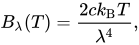


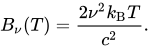
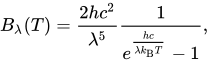

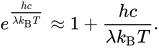
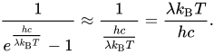



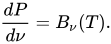







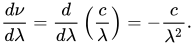
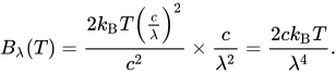
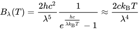
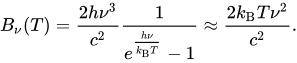




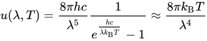



.jpg)


.jpg)


