Feynman diagram

From Wikipedia, the free encyclopedia

https://en.wikipedia.org/wiki/Feynman_diagram 

In this Feynman diagram, an electron (e⁻) and a positron (e⁺) annihilate, producing a photon (γ, represented by the blue sine wave) that becomes a quark–antiquark pair (quark q, antiquark q̄), after which the antiquark radiates a gluon (g, represented by the green helix).

In theoretical physics, a Feynman diagram is a pictorial representation of the mathematical expressions describing the behavior and interaction of subatomic particles. The scheme is named after American physicist Richard Feynman, who introduced the diagrams in 1948.

The calculation of probability amplitudes in theoretical particle physics requires the use of large, complicated integrals over a large number of variables. Feynman diagrams instead represent these integrals graphically.

Feynman diagrams give a simple visualization of what would otherwise be an arcane and abstract formula. According to David Kaiser, "Since the middle of the 20th century, theoretical physicists have increasingly turned to this tool to help them undertake critical calculations. Feynman diagrams have revolutionized nearly every aspect of theoretical physics."

While the diagrams apply primarily to quantum field theory, they can be used in other areas of physics, such as solid-state theory. Frank Wilczek wrote that the calculations that won him the 2004 Nobel Prize in Physics "would have been literally unthinkable without Feynman diagrams, as would [Wilczek's] calculations that established a route to production and observation of the Higgs particle."

A Feynman diagram is a graphical representation of a perturbative contribution to the transition amplitude or correlation function of a quantum mechanical or statistical field theory. Within the canonical formulation of quantum field theory, a Feynman diagram represents a term in the Wick's expansion of the perturbative S-matrix. Alternatively, the path integral formulation of quantum field theory represents the transition amplitude as a weighted sum of all possible histories of the system from the initial to the final state, in terms of either particles or fields. The transition amplitude is then given as the matrix element of the S-matrix between the initial and final states of the quantum system.

Feynman used Ernst Stueckelberg's interpretation of the positron as if it were an electron moving backward in time. Thus, antiparticles are represented as moving backward along the time axis in Feynman diagrams.

Motivation and history

Richard Feynman in 1984

In this diagram, a kaon, made of an up quark and strange antiquark, decays both weakly and strongly into three pions, with intermediate steps involving a W boson and a gluon, represented by the blue sine wave and green spiral, respectively.

When calculating scattering cross-sections in particle physics, the interaction between particles can be described by starting from a free field that describes the incoming and outgoing particles, and including an interaction Hamiltonian to describe how the particles deflect one another. The amplitude for scattering is the sum of each possible interaction history over all possible intermediate particle states. The number of times the interaction Hamiltonian acts is the order of the perturbation expansion, and the time-dependent perturbation theory for fields is known as the Dyson series. When the intermediate states at intermediate times are energy eigenstates (collections of particles with a definite momentum) the series is called old-fashioned perturbation theory (or time-dependent/time-ordered perturbation theory).

The Dyson series can be alternatively rewritten as a sum over Feynman diagrams, where at each vertex both the energy and momentum are conserved, but where the length of the energy-momentum four-vector is not necessarily equal to the mass, i.e. the intermediate particles are so-called off-shell. The Feynman diagrams are much easier to keep track of than "old-fashioned" terms, because the old-fashioned way treats the particle and antiparticle contributions as separate. Each Feynman diagram is the sum of exponentially many old-fashioned terms, because each internal line can separately represent either a particle or an antiparticle. In a non-relativistic classical theory, there are no antiparticles and there is no doubling, so each Feynman diagram includes only one term.

Feynman gave a prescription for calculating the amplitude (the Feynman rules, below) for any given diagram from a field theory Lagrangian. Each internal line corresponds to a factor of the virtual particle's propagator; each vertex where lines meet gives a factor derived from an interaction term in the Lagrangian, and incoming and outgoing lines carry an energy, momentum, and spin.

In addition to their value as a mathematical tool, Feynman diagrams provide deep physical insight into the nature of particle interactions. Particles interact in every way available; in fact, intermediate virtual particles are allowed to propagate faster than light. The probability of each final state is then obtained by summing over all such possibilities. This is closely tied to the functional integral formulation of quantum mechanics, also invented by Feynman—see path integral formulation.

The naïve application of such calculations often produces diagrams whose amplitudes are infinite, because the short-distance particle interactions require a careful limiting procedure, to include particle self-interactions. The technique of renormalization, suggested by Ernst Stueckelberg and Hans Bethe and implemented by Dyson, Feynman, Schwinger, and Tomonaga compensates for this effect and eliminates the troublesome infinities. After renormalization, calculations using Feynman diagrams match experimental results with very high accuracy.

Feynman diagram and path integral methods are also used in statistical mechanics and can even be applied to classical mechanics.

Alternate names

Murray Gell-Mann always referred to Feynman diagrams as Stueckelberg diagrams, after Swiss physicist Ernst Stueckelberg, who devised a similar notation many years earlier. Stueckelberg was motivated by the need for a manifestly covariant formalism for quantum field theory, but did not provide as automated a way to handle symmetry factors and loops, although he was first to find the correct physical interpretation in terms of forward and backward in time particle paths, all without the path-integral.

Historically, as a book-keeping device of covariant perturbation theory, the graphs were called Feynman–Dyson diagrams or Dyson graphs, because the path integral was unfamiliar when they were introduced, and Freeman Dyson's derivation from old-fashioned perturbation theory borrowed from the perturbative expansions in statistical mechanics was easier to follow for physicists trained in earlier methods. Feynman had to lobby hard for the diagrams, which confused physicists trained in equations and graphs.

Representation of physical reality

In their presentations of fundamental interactions,^[8][9] written from the particle physics perspective, Gerard 't Hooft and Martinus Veltman gave good arguments for taking the original, non-regularized Feynman diagrams as the most succinct representation of the physics of quantum scattering of fundamental particles. Their motivations are consistent with the convictions of James Daniel Bjorken and Sidney Drell:

The Feynman graphs and rules of calculation summarize quantum field theory in a form in close contact with the experimental numbers one wants to understand. Although the statement of the theory in terms of graphs may imply perturbation theory, use of graphical methods in the many-body problem shows that this formalism is flexible enough to deal with phenomena of nonperturbative characters ... Some modification of the Feynman rules of calculation may well outlive the elaborate mathematical structure of local canonical quantum field theory ...

In quantum field theories, Feynman diagrams are obtained from a Lagrangian by Feynman rules.

Dimensional regularization is a method for regularizing integrals in the evaluation of Feynman diagrams; it assigns values to them that are meromorphic functions of an auxiliary complex parameter d, called the dimension. Dimensional regularization writes a Feynman integral as an integral depending on the spacetime dimension d and spacetime points.

Particle-path interpretation

A Feynman diagram is a representation of quantum field theory processes in terms of particle interactions. The particles are represented by the diagram lines. The lines can be squiggly or straight, with an arrow or without, depending on the type of particle. A point where lines connect to other lines is a vertex, and this is where the particles meet and interact. The interactions are: emit/absorb particles, deflect particles, or change particle type.

The three different types of lines are: internal lines, connecting vertices; incoming lines, extending from "the past" to a vertex, representing an initial state; and outgoing lines, extending from a vertex to "the future", representing the end state (the latter two are also known as external lines). Traditionally, the bottom of the diagram is the past and the top the future; alternatively, the past is to the left and the future to the right. When calculating correlation functions instead of scattering amplitudes, past and future are not relevant and all lines are internal. The particles then begin and end on small x's, which represent the positions of the operators whose correlation is calculated.

Feynman diagrams are a pictorial representation of a contribution to the total amplitude for a process that can happen in different ways. When a group of incoming particles scatter off each other, the process can be thought of as one where the particles travel over all possible paths, including paths that go backward in time.

Feynman diagrams are graphs that represent the interaction of particles rather than the physical position of the particle during a scattering process. They are not the same as spacetime diagrams and bubble chamber images even though they all describe particle scattering. Unlike a bubble chamber picture, only the sum of all relevant Feynman diagrams represent any given particle interaction; particles do not choose a particular diagram each time they interact. The law of summation is in accord with the principle of superposition—every diagram contributes to the total process's amplitude.

Description

General features of the scattering process A + B → C + D:
• internal lines (red) for intermediate particles and processes, which has a propagator factor ("prop"), external lines (orange) for incoming/outgoing particles to/from vertices (black),
• at each vertex there is 4-momentum conservation using delta functions, 4-momenta entering the vertex are positive while those leaving are negative, the factors at each vertex and internal line are multiplied in the amplitude integral,
• space x and time t axes are not always shown, directions of external lines correspond to passage of time.

A Feynman diagram represents a perturbative contribution to the amplitude of a quantum transition from some initial quantum state to some final quantum state.

For example, in the process of electron-positron annihilation the initial state is one electron and one positron, while the final state is two photons.

Conventionally, the initial state is at the left of the diagram and the final state at the right (although other layouts are also used).

The particles in the initial state are depicted by lines pointing in the direction of the initial state (e.g., to the left). The particles in the final state are represented by lines pointing in the direction of the final state (e.g., to the right).

QED involves two types of particles: matter particles such as electrons or positrons (called fermions) and exchange particles (called gauge bosons). They are represented in Feynman diagrams as follows:

• Electron in the initial state is represented by a solid line, with an arrow indicating the spin of the particle e.g. pointing toward the vertex (→•).
• Electron in the final state is represented by a line, with an arrow indicating the spin of the particle e.g. pointing away from the vertex: (•→).
• Positron in the initial state is represented by a solid line, with an arrow indicating the spin of the particle e.g. pointing away from the vertex: (←•).
• Positron in the final state is represented by a line, with an arrow indicating the spin of the particle e.g. pointing toward the vertex: (•←).
• Virtual Photon in the initial and the final states is represented by a wavy line (~• and •~).

In QED each vertex has three lines attached to it: one bosonic line, one fermionic line with arrow toward the vertex, and one fermionic line with arrow away from the vertex.

Vertices can be connected by a bosonic or fermionic propagator. A bosonic propagator is represented by a wavy line connecting two vertices (•~•). A fermionic propagator is represented by a solid line with an arrow connecting two vertices, (•←•).

The number of vertices gives the order of the term in the perturbation series expansion of the transition amplitude.

Electron–positron annihilation example

Feynman diagram of electron/positron annihilation with the time axis vertical

The electron–positron annihilation interaction:

e⁺ + e⁻ → 2γ

has a contribution from the second order Feynman diagram:

In the initial state (at the bottom; early time) there is one electron (e⁻) and one positron (e⁺) and in the final state (at the top; late time) there are two photons (γ).

Canonical quantization formulation

The probability amplitude for a transition of a quantum system (between asymptotically free states) from the initial state |i⟩ to the final state | f ⟩ is given by the matrix element

${\displaystyle S_{\mathrm{f}\mathrm{i}}=⟨\mathrm{f}|S|\mathrm{i}⟩,}$

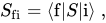
where S is the S-matrix. In terms of the time-evolution operator U, it is simply

${\displaystyle S=\underset{t_2\to +\mathrm{\infty }}{lim}\left[\underset{t_1\to -\mathrm{\infty }}{lim}U(t_2,t_1)\right].}$

In the interaction picture, this expands to

${\displaystyle S=\mathcal{T}\exp \left(-i{\int }_{-\mathrm{\infty }}^{+\mathrm{\infty }}d\tau H_V(\tau )\right).}$

where H_V is the interaction Hamiltonian and ${\displaystyle \mathcal{T}}$ signifies the time-ordered product of operators. Dyson's formula expands the time-ordered matrix exponential into a perturbation series in the powers of the interaction Hamiltonian density,

${\displaystyle S=\sum _{n=0}^{\mathrm{\infty }}\frac{(-i{)}^n}{n!}\left(\prod _{j=1}^n\int d^4{x}_j\right)\mathcal{T}\left\{\prod _{j=1}^n{\mathcal{H}}_V\left(x_j\right)\right\}\equiv \sum _{n=0}^{\mathrm{\infty }}{S}^{(n)}.}$

Equivalently, with the interaction Lagrangian L_V, it is

${\displaystyle S=\sum _{n=0}^{\mathrm{\infty }}\frac{i^n}{n!}\left(\prod _{j=1}^n\int d^4{x}_j\right)\mathcal{T}\left\{\prod _{j=1}^n{\mathcal{L}}_V\left(x_j\right)\right\}\equiv \sum _{n=0}^{\mathrm{\infty }}{S}^{(n)}.}$

A Feynman diagram is a graphical representation of a single summand in the Wick's expansion of the time-ordered product in the nth-order term S⁽ⁿ⁾ of the Dyson series of the S-matrix,

${\displaystyle \mathcal{T}\prod _{j=1}^n{\mathcal{L}}_V\left(x_j\right)=\sum _{\text{A}}(\pm )\mathcal{N}\prod _{j=1}^n{\mathcal{L}}_V\left(x_j\right),}$

where N signifies the normal-ordered product of the operators and (±) takes care of the possible sign change when commuting the fermionic operators to bring them together for a contraction (a propagator) and A represents all possible contractions.

Feynman rules

The diagrams are drawn according to the Feynman rules, which depend upon the interaction Lagrangian. For the QED interaction Lagrangian

${\displaystyle L_v=-g\overline{\psi }{\gamma }^{\mu }\psi A_{\mu }}$

describing the interaction of a fermionic field ψ with a bosonic gauge field A_μ, the Feynman rules can be formulated in coordinate space as follows:

• Each integration coordinate x_j is represented by a point (sometimes called a vertex);
• A bosonic propagator is represented by a wiggly line connecting two points;
• A fermionic propagator is represented by a solid line connecting two points;
• A bosonic field ${\displaystyle A_{\mu }(x_i)}$ is represented by a wiggly line attached to the point x_i;
• A fermionic field ψ(x_i) is represented by a solid line attached to the point x_i with an arrow toward the point;
• An anti-fermionic field ψ(x_i) is represented by a solid line attached to the point x_i with an arrow away from the point;

Example: second order processes in QED

The second order perturbation term in the S-matrix is

${\displaystyle S^{(2)}=\frac{(ie{)}^2}{2!}\int d^{4}x{d}^4{x}^{\prime }T\overline{\psi }(x){\gamma }^{\mu }\psi (x)A_{\mu }(x)\overline{\psi }(x^{\prime }){\gamma }^{\nu }\psi (x^{\prime })A_{\nu }(x^{\prime }).}$

Scattering of fermions

The Feynman diagram of the term ${\displaystyle N\overline{\psi }(x)ie{\gamma }^{\mu }\psi (x)\overline{\psi }(x^{\prime })ie{\gamma }^{\nu }\psi (x^{\prime })A_{\mu }(x)A_{\nu }(x^{\prime })}$

The Wick's expansion of the integrand gives (among others) the following term

${\displaystyle N\overline{\psi }(x){\gamma }^{\mu }\psi (x)\overline{\psi }(x^{\prime }){\gamma }^{\nu }\psi (x^{\prime })\underset{\_}{A_{\mu }(x)A_{\nu }(x^{\prime })},}$

where

${\displaystyle \underset{\_}{A_{\mu }(x)A_{\nu }(x^{\prime })}=\int \frac{d^{4}k}{(2\pi {)}^4}\frac{-i{g}_{\mu \nu }}{k^2+i0}{e}^{-ik(x-x^{\prime })}}$

is the electromagnetic contraction (propagator) in the Feynman gauge. This term is represented by the Feynman diagram at the right. This diagram gives contributions to the following processes:

1. e⁻ e⁻ scattering (initial state at the right, final state at the left of the diagram);
2. e⁺ e⁺ scattering (initial state at the left, final state at the right of the diagram);
3. e⁻ e⁺ scattering (initial state at the bottom/top, final state at the top/bottom of the diagram).

Compton scattering and annihilation/generation of e⁻ e⁺ pairs

Another interesting term in the expansion is

${\displaystyle N\overline{\psi }(x){\gamma }^{\mu }\underset{\_}{\psi (x)\overline{\psi }(x^{\prime })}{\gamma }^{\nu }\psi (x^{\prime })A_{\mu }(x)A_{\nu }(x^{\prime }),}$

where

${\displaystyle \underset{\_}{\psi (x)\overline{\psi }(x^{\prime })}=\int \frac{d^{4}p}{(2\pi {)}^4}\frac{i}{\gamma p-m+i0}{e}^{-ip(x-x^{\prime })}}$

is the fermionic contraction (propagator).

Path integral formulation

In a path integral, the field Lagrangian, integrated over all possible field histories, defines the probability amplitude to go from one field configuration to another. In order to make sense, the field theory must have a well-defined ground state, and the integral must be performed a little bit rotated into imaginary time, i.e. a Wick rotation. The path integral formalism is completely equivalent to the canonical operator formalism above.

Scalar field Lagrangian

A simple example is the free relativistic scalar field in d dimensions, whose action integral is:

${\displaystyle S=\int \frac{1}{2}{\mathrm{\partial }}_{\mu }\varphi {\mathrm{\partial }}^{\mu }\varphi d^{d}x.}$

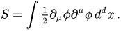
The probability amplitude for a process is:

${\displaystyle {\int }_A^B{e}^{iS}D\varphi ,}$

where A and B are space-like hypersurfaces that define the boundary conditions. The collection of all the φ(A) on the starting hypersurface give the field's initial value, analogous to the starting position for a point particle, and the field values φ(B) at each point of the final hypersurface defines the final field value, which is allowed to vary, giving a different amplitude to end up at different values. This is the field-to-field transition amplitude.

The path integral gives the expectation value of operators between the initial and final state:

${\displaystyle {\int }_A^B{e}^{iS}\varphi (x_1)\cdots \varphi (x_n)D\varphi =⟨A\left|\varphi (x_1)\cdots \varphi (x_n)\right|B⟩,}$

and in the limit that A and B recede to the infinite past and the infinite future, the only contribution that matters is from the ground state (this is only rigorously true if the path-integral is defined slightly rotated into imaginary time). The path integral can be thought of as analogous to a probability distribution, and it is convenient to define it so that multiplying by a constant does not change anything:

${\displaystyle \frac{{\displaystyle \int e^{iS}\varphi (x_1)\cdots \varphi (x_n)D\varphi }}{{\displaystyle \int e^{iS}D\varphi }}=⟨0\left|\varphi (x_1)\cdots \varphi (x_n)\right|0⟩.}$

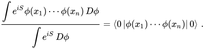
The field's partition function is the normalization factor on the bottom, which coincides with the statistical mechanical partition function at zero temperature when rotated into imaginary time.

The initial-to-final amplitudes are ill-defined if one thinks of the continuum limit right from the beginning, because the fluctuations in the field can become unbounded. So the path-integral can be thought of as on a discrete square lattice, with lattice spacing a and the limit a → 0 should be taken carefully. If the final results do not depend on the shape of the lattice or the value of a, then the continuum limit exists.

On a lattice

On a lattice, (i), the field can be expanded in Fourier modes:

${\displaystyle \varphi (x)=\int \frac{dk}{(2\pi {)}^d}\varphi (k)e^{ik\cdot x}={\int }_k\varphi (k)e^{ikx}.}$

Here the integration domain is over k restricted to a cube of side length ⁠2π/a⁠, so that large values of k are not allowed. It is important to note that the k-measure contains the factors of 2π from Fourier transforms, this is the best standard convention for k-integrals in QFT. The lattice means that fluctuations at large k are not allowed to contribute right away, they only start to contribute in the limit a → 0. Sometimes, instead of a lattice, the field modes are just cut off at high values of k instead.

It is also convenient from time to time to consider the space-time volume to be finite, so that the k modes are also a lattice. This is not strictly as necessary as the space-lattice limit, because interactions in k are not localized, but it is convenient for keeping track of the factors in front of the k-integrals and the momentum-conserving delta functions that will arise.

On a lattice, (ii), the action needs to be discretized:

${\displaystyle S=\sum _{⟨x,y⟩}\frac{1}{2}(\varphi (x)-\varphi (y){)}^2,}$

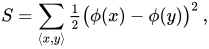
where ⟨x,y⟩ is a pair of nearest lattice neighbors x and y. The discretization should be thought of as defining what the derivative ∂_μφ means.

In terms of the lattice Fourier modes, the action can be written:

${\displaystyle S={\int }_k((1-\cos (k_1))+(1-\cos (k_2))+\cdots +(1-\cos (k_d))){\varphi }_k^{\ast }{\varphi }^k.}$

For k near zero this is:

${\displaystyle S={\int }_k\frac{1}{2}{k}^2{\left|\varphi (k)\right|}^2.}$

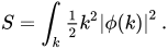
Now we have the continuum Fourier transform of the original action. In finite volume, the quantity d^dk is not infinitesimal, but becomes the volume of a box made by neighboring Fourier modes, or (⁠2π/V⁠)^d
 .

The field φ is real-valued, so the Fourier transform obeys:

${\displaystyle \varphi (k{)}^{\ast }=\varphi (-k).}$

In terms of real and imaginary parts, the real part of φ(k) is an even function of k, while the imaginary part is odd. The Fourier transform avoids double-counting, so that it can be written:

${\displaystyle S={\int }_k\frac{1}{2}{k}^2\varphi (k)\varphi (-k)}$

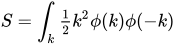
over an integration domain that integrates over each pair (k,−k) exactly once.

For a complex scalar field with action

${\displaystyle S=\int \frac{1}{2}{\mathrm{\partial }}_{\mu }{\varphi }^{\ast }{\mathrm{\partial }}^{\mu }\varphi d^{d}x}$

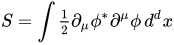
the Fourier transform is unconstrained:

${\displaystyle S={\int }_k\frac{1}{2}{k}^2{\left|\varphi (k)\right|}^2}$

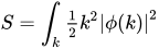
and the integral is over all k.

Integrating over all different values of φ(x) is equivalent to integrating over all Fourier modes, because taking a Fourier transform is a unitary linear transformation of field coordinates. When you change coordinates in a multidimensional integral by a linear transformation, the value of the new integral is given by the determinant of the transformation matrix. If

${\displaystyle y_i=A_{ij}{x}_j,}$

then

${\displaystyle det(A)\int d{x}_{1}d{x}_2\cdots d{x}_n=\int d{y}_{1}d{y}_2\cdots d{y}_n.}$

If A is a rotation, then

${\displaystyle A^{\mathrm{T}}A=I}$

so that det A = ±1, and the sign depends on whether the rotation includes a reflection or not.

The matrix that changes coordinates from φ(x) to φ(k) can be read off from the definition of a Fourier transform.

${\displaystyle A_{kx}=e^{ikx}}$

and the Fourier inversion theorem tells you the inverse:

${\displaystyle A_{kx}^{-1}=e^{-ikx}}$

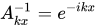
which is the complex conjugate-transpose, up to factors of 2π. On a finite volume lattice, the determinant is nonzero and independent of the field values.

${\displaystyle detA=1}$

and the path integral is a separate factor at each value of k.

${\displaystyle \int \exp \left(\frac{i}{2}\sum _k{k}^2{\varphi }^{\ast }(k)\varphi (k)\right)D\varphi =\prod _k{\int }_{{\varphi }_k}{e}^{\frac{i}{2}{k}^2{\left|{\varphi }_k\right|}^2{d}^{d}k}}$

The factor d^dk is the infinitesimal volume of a discrete cell in k-space, in a square lattice box

${\displaystyle d^{d}k={\left(\frac{1}{L}\right)}^d,}$

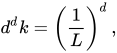
where L is the side-length of the box. Each separate factor is an oscillatory Gaussian, and the width of the Gaussian diverges as the volume goes to infinity.

In imaginary time, the Euclidean action becomes positive definite, and can be interpreted as a probability distribution. The probability of a field having values φ_k is

${\displaystyle e^{{\int }_k-\frac{1}{2}{k}^2{\varphi }_k^{\ast }{\varphi }_k}=\prod _k{e}^{-k^2{\left|{\varphi }_k\right|}^2{d}^{d}k}.}$

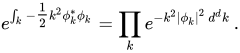
The expectation value of the field is the statistical expectation value of the field when chosen according to the probability distribution:

${\displaystyle ⟨\varphi (x_1)\cdots \varphi (x_n)⟩=\frac{{\displaystyle \int e^{-S}\varphi (x_1)\cdots \varphi (x_n)D\varphi }}{{\displaystyle \int e^{-S}D\varphi }}}$

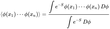
Since the probability of φ_k is a product, the value of φ_k at each separate value of k is independently Gaussian distributed. The variance of the Gaussian is ⁠1/k²d^dk⁠, which is formally infinite, but that just means that the fluctuations are unbounded in infinite volume. In any finite volume, the integral is replaced by a discrete sum, and the variance of the integral is ⁠V/k²⁠.

Monte Carlo

The path integral defines a probabilistic algorithm to generate a Euclidean scalar field configuration. Randomly pick the real and imaginary parts of each Fourier mode at wavenumber k to be a Gaussian random variable with variance ⁠1/k²⁠. This generates a configuration φ_C(k) at random, and the Fourier transform gives φ_C(x). For real scalar fields, the algorithm must generate only one of each pair φ(k), φ(−k), and make the second the complex conjugate of the first.

To find any correlation function, generate a field again and again by this procedure, and find the statistical average:

${\displaystyle ⟨\varphi (x_1)\cdots \varphi (x_n)⟩=\underset{|C|\to \mathrm{\infty }}{lim}\frac{{\displaystyle \sum _C{\varphi }_C(x_1)\cdots {\varphi }_C(x_n)}}{|C|}}$

where |C| is the number of configurations, and the sum is of the product of the field values on each configuration. The Euclidean correlation function is just the same as the correlation function in statistics or statistical mechanics. The quantum mechanical correlation functions are an analytic continuation of the Euclidean correlation functions.

For free fields with a quadratic action, the probability distribution is a high-dimensional Gaussian, and the statistical average is given by an explicit formula. But the Monte Carlo method also works well for bosonic interacting field theories where there is no closed form for the correlation functions.

Scalar propagator

Each mode is independently Gaussian distributed. The expectation of field modes is easy to calculate:

${\displaystyle ⟨{\varphi }_k{\varphi }_{k^{\prime }}⟩=0}$

for k ≠ k′, since then the two Gaussian random variables are independent and both have zero mean.

${\displaystyle ⟨{\varphi }_k{\varphi }_k⟩=\frac{V}{k^2}}$

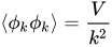
in finite volume V, when the two k-values coincide, since this is the variance of the Gaussian. In the infinite volume limit,

${\displaystyle ⟨\varphi (k)\varphi (k^{\prime })⟩=\delta (k-k^{\prime })\frac{1}{k^2}}$

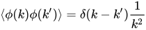
Strictly speaking, this is an approximation: the lattice propagator is:

${\displaystyle ⟨\varphi (k)\varphi (k^{\prime })⟩=\delta (k-k^{\prime })\frac{1}{2(d-\cos (k_1)+\cos (k_2)\cdots +\cos (k_d))}}$

But near k = 0, for field fluctuations long compared to the lattice spacing, the two forms coincide.

The delta functions contain factors of 2π, so that they cancel out the 2π factors in the measure for k integrals.

${\displaystyle \delta (k)=(2\pi {)}^d{\delta }_D(k_1){\delta }_D(k_2)\cdots {\delta }_D(k_d)}$

where δ_D(k) is the ordinary one-dimensional Dirac delta function. This convention for delta-functions is not universal—some authors keep the factors of 2π in the delta functions (and in the k-integration) explicit.

Equation of motion

The form of the propagator can be more easily found by using the equation of motion for the field. From the Lagrangian, the equation of motion is:

${\displaystyle {\mathrm{\partial }}_{\mu }{\mathrm{\partial }}^{\mu }\varphi =0}$

and in an expectation value, this says:

${\displaystyle {\mathrm{\partial }}_{\mu }{\mathrm{\partial }}^{\mu }⟨\varphi (x)\varphi (y)⟩=0}$

Where the derivatives act on x, and the identity is true everywhere except when x and y coincide, and the operator order matters. The form of the singularity can be understood from the canonical commutation relations to be a delta-function. Defining the (Euclidean) Feynman propagator Δ as the Fourier transform of the time-ordered two-point function (the one that comes from the path-integral):

${\displaystyle {\mathrm{\partial }}^2\mathrm{\Delta }(x)=i\delta (x)}$

So that:

${\displaystyle \mathrm{\Delta }(k)=\frac{i}{k^2}}$

If the equations of motion are linear, the propagator will always be the reciprocal of the quadratic-form matrix that defines the free Lagrangian, since this gives the equations of motion. This is also easy to see directly from the path integral. The factor of i disappears in the Euclidean theory.

Wick theorem

Main article: Wick's theorem

Because each field mode is an independent Gaussian, the expectation values for the product of many field modes obeys Wick's theorem:

${\displaystyle ⟨\varphi (k_1)\varphi (k_2)\cdots \varphi (k_n)⟩}$

is zero unless the field modes coincide in pairs. This means that it is zero for an odd number of φ, and for an even number of φ, it is equal to a contribution from each pair separately, with a delta function.

${\displaystyle ⟨\varphi (k_1)\cdots \varphi (k_{2n})⟩=\sum \prod _{i,j}\frac{\delta \left(k_i-k_j\right)}{k_i^2}}$

where the sum is over each partition of the field modes into pairs, and the product is over the pairs. For example,

${\displaystyle ⟨\varphi (k_1)\varphi (k_2)\varphi (k_3)\varphi (k_4)⟩=\frac{\delta (k_1-k_2)}{k_1^2}\frac{\delta (k_3-k_4)}{k_3^2}+\frac{\delta (k_1-k_3)}{k_3^2}\frac{\delta (k_2-k_4)}{k_2^2}+\frac{\delta (k_1-k_4)}{k_1^2}\frac{\delta (k_2-k_3)}{k_2^2}}$

An interpretation of Wick's theorem is that each field insertion can be thought of as a dangling line, and the expectation value is calculated by linking up the lines in pairs, putting a delta function factor that ensures that the momentum of each partner in the pair is equal, and dividing by the propagator.

Higher Gaussian moments — completing Wick's theorem

There is a subtle point left before Wick's theorem is proved—what if more than two of the ${\displaystyle \varphi }$s have the same momentum? If it's an odd number, the integral is zero; negative values cancel with the positive values. But if the number is even, the integral is positive. The previous demonstration assumed that the ${\displaystyle \varphi }$s would only match up in pairs.

But the theorem is correct even when arbitrarily many of the ${\displaystyle \varphi }$ are equal, and this is a notable property of Gaussian integration:

${\displaystyle I=\int e^{-a{x}^2/2}dx=\sqrt{\frac{2\pi }{a}}}$

${\displaystyle \frac{{\mathrm{\partial }}^n}{\mathrm{\partial }{a}^n}I=\int \frac{x^{2n}}{2^n}{e}^{-a{x}^2/2}dx=\frac{1\cdot 3\cdot 5\dots \cdot (2n-1)}{2\cdot 2\cdot 2\dots \cdot 2}\sqrt{2\pi }{a}^{-\frac{2n+1}{2}}}$

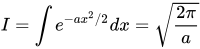
Dividing by I,

${\displaystyle ⟨x^{2n}⟩=\frac{{\displaystyle \int x^{2n}{e}^{-a{x}^2/2}}}{{\displaystyle \int e^{-a{x}^2/2}}}=1\cdot 3\cdot 5\dots \cdot (2n-1)\frac{1}{a^n}}$

${\displaystyle ⟨x^2⟩=\frac{1}{a}}$

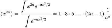
If Wick's theorem were correct, the higher moments would be given by all possible pairings of a list of 2n different x:

${\displaystyle ⟨x_1{x}_2{x}_3\cdots x_{2n}⟩}$

where the x are all the same variable, the index is just to keep track of the number of ways to pair them. The first x can be paired with 2n − 1 others, leaving 2n − 2. The next unpaired x can be paired with 2n − 3 different x leaving 2n − 4, and so on. This means that Wick's theorem, uncorrected, says that the expectation value of x²ⁿ should be:

${\displaystyle ⟨x^{2n}⟩=(2n-1)\cdot (2n-3)\dots \cdot 5\cdot 3\cdot 1{⟨x^2⟩}^n}$

and this is in fact the correct answer. So Wick's theorem holds no matter how many of the momenta of the internal variables coincide.

Interaction

Interactions are represented by higher order contributions, since quadratic contributions are always Gaussian. The simplest interaction is the quartic self-interaction, with an action:

${\displaystyle S=\int {\mathrm{\partial }}^{\mu }\varphi {\mathrm{\partial }}_{\mu }\varphi +\frac{\lambda }{4!}{\varphi }^4.}$

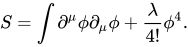
The reason for the combinatorial factor 4! will be clear soon. Writing the action in terms of the lattice (or continuum) Fourier modes:

${\displaystyle S={\int }_k{k}^2{\left|\varphi (k)\right|}^2+\frac{\lambda }{4!}{\int }_{k_1{k}_2{k}_3{k}_4}\varphi (k_1)\varphi (k_2)\varphi (k_3)\varphi (k_4)\delta (k_1+k_2+k_3+k_4)=S_F+X.}$

Where S_F is the free action, whose correlation functions are given by Wick's theorem. The exponential of S in the path integral can be expanded in powers of λ, giving a series of corrections to the free action.

${\displaystyle e^{-S}=e^{-S_F}\left(1+X+\frac{1}{2!}XX+\frac{1}{3!}XXX+\cdots \right)}$

The path integral for the interacting action is then a power series of corrections to the free action. The term represented by X should be thought of as four half-lines, one for each factor of φ(k). The half-lines meet at a vertex, which contributes a delta-function that ensures that the sum of the momenta are all equal.

To compute a correlation function in the interacting theory, there is a contribution from the X terms now. For example, the path-integral for the four-field correlator:

${\displaystyle ⟨\varphi (k_1)\varphi (k_2)\varphi (k_3)\varphi (k_4)⟩=\frac{{\displaystyle \int e^{-S}\varphi (k_1)\varphi (k_2)\varphi (k_3)\varphi (k_4)D\varphi }}{Z}}$

which in the free field was only nonzero when the momenta k were equal in pairs, is now nonzero for all values of k. The momenta of the insertions φ(k_i) can now match up with the momenta of the Xs in the expansion. The insertions should also be thought of as half-lines, four in this case, which carry a momentum k, but one that is not integrated.

The lowest-order contribution comes from the first nontrivial term e^−S_FX in the Taylor expansion of the action. Wick's theorem requires that the momenta in the X half-lines, the φ(k) factors in X, should match up with the momenta of the external half-lines in pairs. The new contribution is equal to:

${\displaystyle \lambda \frac{1}{k_1^2}\frac{1}{k_2^2}\frac{1}{k_3^2}\frac{1}{k_4^2}.}$

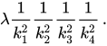
The 4! inside X is canceled because there are exactly 4! ways to match the half-lines in X to the external half-lines. Each of these different ways of matching the half-lines together in pairs contributes exactly once, regardless of the values of k_1,2,3,4, by Wick's theorem.

Feynman diagrams

The expansion of the action in powers of X gives a series of terms with progressively higher number of Xs. The contribution from the term with exactly n Xs is called nth order.

The nth order terms has:

1. 4n internal half-lines, which are the factors of φ(k) from the Xs. These all end on a vertex, and are integrated over all possible k.
2. external half-lines, which are the come from the φ(k) insertions in the integral.

By Wick's theorem, each pair of half-lines must be paired together to make a line, and this line gives a factor of

${\displaystyle \frac{\delta (k_1+k_2)}{k_1^2}}$

which multiplies the contribution. This means that the two half-lines that make a line are forced to have equal and opposite momentum. The line itself should be labelled by an arrow, drawn parallel to the line, and labeled by the momentum in the line k. The half-line at the tail end of the arrow carries momentum k, while the half-line at the head-end carries momentum −k. If one of the two half-lines is external, this kills the integral over the internal k, since it forces the internal k to be equal to the external k. If both are internal, the integral over k remains.

The diagrams that are formed by linking the half-lines in the Xs with the external half-lines, representing insertions, are the Feynman diagrams of this theory. Each line carries a factor of ⁠1/k²⁠, the propagator, and either goes from vertex to vertex, or ends at an insertion. If it is internal, it is integrated over. At each vertex, the total incoming k is equal to the total outgoing k.

The number of ways of making a diagram by joining half-lines into lines almost completely cancels the factorial factors coming from the Taylor series of the exponential and the 4! at each vertex.

Loop order

A forest diagram is one where all the internal lines have momentum that is completely determined by the external lines and the condition that the incoming and outgoing momentum are equal at each vertex. The contribution of these diagrams is a product of propagators, without any integration. A tree diagram is a connected forest diagram.

An example of a tree diagram is the one where each of four external lines end on an X. Another is when three external lines end on an X, and the remaining half-line joins up with another X, and the remaining half-lines of this X run off to external lines. These are all also forest diagrams (as every tree is a forest); an example of a forest that is not a tree is when eight external lines end on two Xs.

It is easy to verify that in all these cases, the momenta on all the internal lines is determined by the external momenta and the condition of momentum conservation in each vertex.

A diagram that is not a forest diagram is called a loop diagram, and an example is one where two lines of an X are joined to external lines, while the remaining two lines are joined to each other. The two lines joined to each other can have any momentum at all, since they both enter and leave the same vertex. A more complicated example is one where two Xs are joined to each other by matching the legs one to the other. This diagram has no external lines at all.

The reason loop diagrams are called loop diagrams is because the number of k-integrals that are left undetermined by momentum conservation is equal to the number of independent closed loops in the diagram, where independent loops are counted as in homology theory. The homology is real-valued (actually R^d valued), the value associated with each line is the momentum. The boundary operator takes each line to the sum of the end-vertices with a positive sign at the head and a negative sign at the tail. The condition that the momentum is conserved is exactly the condition that the boundary of the k-valued weighted graph is zero.

A set of valid k-values can be arbitrarily redefined whenever there is a closed loop. A closed loop is a cyclical path of adjacent vertices that never revisits the same vertex. Such a cycle can be thought of as the boundary of a hypothetical 2-cell. The k-labellings of a graph that conserve momentum (i.e. which has zero boundary) up to redefinitions of k (i.e. up to boundaries of 2-cells) define the first homology of a graph. The number of independent momenta that are not determined is then equal to the number of independent homology loops. For many graphs, this is equal to the number of loops as counted in the most intuitive way.

Symmetry factors

The number of ways to form a given Feynman diagram by joining half-lines is large, and by Wick's theorem, each way of pairing up the half-lines contributes equally. Often, this completely cancels the factorials in the denominator of each term, but the cancellation is sometimes incomplete.

The uncancelled denominator is called the symmetry factor of the diagram. The contribution of each diagram to the correlation function must be divided by its symmetry factor.

For example, consider the Feynman diagram formed from two external lines joined to one X, and the remaining two half-lines in the X joined to each other. There are 4 × 3 ways to join the external half-lines to the X, and then there is only one way to join the two remaining lines to each other. The X comes divided by 4! = 4 × 3 × 2, but the number of ways to link up the X half lines to make the diagram is only 4 × 3, so the contribution of this diagram is divided by two.

For another example, consider the diagram formed by joining all the half-lines of one X to all the half-lines of another X. This diagram is called a vacuum bubble, because it does not link up to any external lines. There are 4! ways to form this diagram, but the denominator includes a 2! (from the expansion of the exponential, there are two Xs) and two factors of 4!. The contribution is multiplied by ⁠4!/2 × 4! × 4!⁠ = ⁠1/48⁠.

Another example is the Feynman diagram formed from two Xs where each X links up to two external lines, and the remaining two half-lines of each X are joined to each other. The number of ways to link an X to two external lines is 4 × 3, and either X could link up to either pair, giving an additional factor of 2. The remaining two half-lines in the two Xs can be linked to each other in two ways, so that the total number of ways to form the diagram is 4 × 3 × 4 × 3 × 2 × 2, while the denominator is 4! × 4! × 2!. The total symmetry factor is 2, and the contribution of this diagram is divided by 2.

The symmetry factor theorem gives the symmetry factor for a general diagram: the contribution of each Feynman diagram must be divided by the order of its group of automorphisms, the number of symmetries that it has.

An automorphism of a Feynman graph is a permutation M of the lines and a permutation N of the vertices with the following properties:

1. If a line l goes from vertex v to vertex v′, then M(l) goes from N(v) to N(v′). If the line is undirected, as it is for a real scalar field, then M(l) can go from N(v′) to N(v) too.
2. If a line l ends on an external line, M(l) ends on the same external line.
3. If there are different types of lines, M(l) should preserve the type.

This theorem has an interpretation in terms of particle-paths: when identical particles are present, the integral over all intermediate particles must not double-count states that differ only by interchanging identical particles.

Proof: To prove this theorem, label all the internal and external lines of a diagram with a unique name. Then form the diagram by linking a half-line to a name and then to the other half line.

Now count the number of ways to form the named diagram. Each permutation of the Xs gives a different pattern of linking names to half-lines, and this is a factor of n!. Each permutation of the half-lines in a single X gives a factor of 4!. So a named diagram can be formed in exactly as many ways as the denominator of the Feynman expansion.

But the number of unnamed diagrams is smaller than the number of named diagram by the order of the automorphism group of the graph.

Connected diagrams: linked-cluster theorem

Roughly speaking, a Feynman diagram is called connected if all vertices and propagator lines are linked by a sequence of vertices and propagators of the diagram itself. If one views it as an undirected graph it is connected. The remarkable relevance of such diagrams in QFTs is due to the fact that they are sufficient to determine the quantum partition function Z[J]. More precisely, connected Feynman diagrams determine

${\displaystyle iW[J]\equiv \ln Z[J].}$

To see this, one should recall that

${\displaystyle Z[J]\propto \sum _k{D}_k}$

with D_k constructed from some (arbitrary) Feynman diagram that can be thought to consist of several connected components C_i. If one encounters n_i (identical) copies of a component C_i within the Feynman diagram D_k one has to include a symmetry factor n_i!. However, in the end each contribution of a Feynman diagram D_k to the partition function has the generic form

${\displaystyle \prod _i\frac{C_i^{n_i}}{n_i!}}$

where i labels the (infinitely) many connected Feynman diagrams possible.

A scheme to successively create such contributions from the D_k to Z[J] is obtained by

${\displaystyle \left(\frac{1}{0!}+\frac{C_1}{1!}+\frac{C_1^2}{2!}+\cdots \right)\left(1+C_2+\frac{1}{2}{C}_2^2+\cdots \right)\cdots }$

and therefore yields

${\displaystyle Z[J]\propto \prod _i\sum _{n_i=0}^{\mathrm{\infty }}\frac{C_i^{n_i}}{n_i!}=\exp \sum _i{C}_i\propto \exp W[J].}$

To establish the normalization Z₀ = exp W[0] = 1 one simply calculates all connected vacuum diagrams, i.e., the diagrams without any sources J (sometimes referred to as external legs of a Feynman diagram).

The linked-cluster theorem was first proved to order four by Keith Brueckner in 1955, and for infinite orders by Jeffrey Goldstone in 1957.

Vacuum bubbles

An immediate consequence of the linked-cluster theorem is that all vacuum bubbles, diagrams without external lines, cancel when calculating correlation functions. A correlation function is given by a ratio of path-integrals:

${\displaystyle ⟨{\varphi }_1(x_1)\cdots {\varphi }_n(x_n)⟩=\frac{{\displaystyle \int e^{-S}{\varphi }_1(x_1)\cdots {\varphi }_n(x_n)D\varphi }}{{\displaystyle \int e^{-S}D\varphi }}.}$

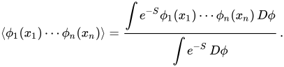
The top is the sum over all Feynman diagrams, including disconnected diagrams that do not link up to external lines at all. In terms of the connected diagrams, the numerator includes the same contributions of vacuum bubbles as the denominator:

${\displaystyle \int e^{-S}{\varphi }_1(x_1)\cdots {\varphi }_n(x_n)D\varphi =\left(\sum E_i\right)\left(\exp \left(\sum _i{C}_i\right)\right).}$

Where the sum over E diagrams includes only those diagrams each of whose connected components end on at least one external line. The vacuum bubbles are the same whatever the external lines, and give an overall multiplicative factor. The denominator is the sum over all vacuum bubbles, and dividing gets rid of the second factor.

The vacuum bubbles then are only useful for determining Z itself, which from the definition of the path integral is equal to:

${\displaystyle Z=\int e^{-S}D\varphi =e^{-HT}=e^{-\rho V}}$

where ρ is the energy density in the vacuum. Each vacuum bubble contains a factor of δ(k) zeroing the total k at each vertex, and when there are no external lines, this contains a factor of δ(0), because the momentum conservation is over-enforced. In finite volume, this factor can be identified as the total volume of space time. Dividing by the volume, the remaining integral for the vacuum bubble has an interpretation: it is a contribution to the energy density of the vacuum.

Sources

Correlation functions are the sum of the connected Feynman diagrams, but the formalism treats the connected and disconnected diagrams differently. Internal lines end on vertices, while external lines go off to insertions. Introducing sources unifies the formalism, by making new vertices where one line can end.

Sources are external fields, fields that contribute to the action, but are not dynamical variables. A scalar field source is another scalar field h that contributes a term to the (Lorentz) Lagrangian:

${\displaystyle \int h(x)\varphi (x)d^{d}x=\int h(k)\varphi (k)d^{d}k}$

In the Feynman expansion, this contributes H terms with one half-line ending on a vertex. Lines in a Feynman diagram can now end either on an X vertex, or on an H vertex, and only one line enters an H vertex. The Feynman rule for an H vertex is that a line from an H with momentum k gets a factor of h(k).

The sum of the connected diagrams in the presence of sources includes a term for each connected diagram in the absence of sources, except now the diagrams can end on the source. Traditionally, a source is represented by a little "×" with one line extending out, exactly as an insertion.

${\displaystyle \log (Z[h])=\sum _{n,C}h(k_1)h(k_2)\cdots h(k_n)C(k_1,\cdots ,k_n)}$

where C(k₁,...,k_n) is the connected diagram with n external lines carrying momentum as indicated. The sum is over all connected diagrams, as before.

The field h is not dynamical, which means that there is no path integral over h: h is just a parameter in the Lagrangian, which varies from point to point. The path integral for the field is:

${\displaystyle Z[h]=\int e^{iS+i\int h\varphi }D\varphi }$

and it is a function of the values of h at every point. One way to interpret this expression is that it is taking the Fourier transform in field space. If there is a probability density on Rⁿ, the Fourier transform of the probability density is:

${\displaystyle \int \rho (y)e^{iky}{d}^{n}y=⟨e^{iky}⟩=⟨\prod _{i=1}^n{e}^{i{h}_i{y}_i}⟩}$

The Fourier transform is the expectation of an oscillatory exponential. The path integral in the presence of a source h(x) is:

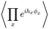
${\displaystyle Z[h]=\int e^{iS}{e}^{i{\int }_{x}h(x)\varphi (x)}D\varphi =⟨e^{ih\varphi }⟩}$

which, on a lattice, is the product of an oscillatory exponential for each field value:

${\displaystyle ⟨\prod _x{e}^{i{h}_x{\varphi }_x}⟩}$

The Fourier transform of a delta-function is a constant, which gives a formal expression for a delta function:

${\displaystyle \delta (x-y)=\int e^{ik(x-y)}dk}$

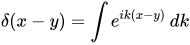
This tells you what a field delta function looks like in a path-integral. For two scalar fields φ and η,

${\displaystyle \delta (\varphi -\eta )=\int e^{ih(x)(\varphi (x)-\eta (x))d^{d}x}Dh,}$

which integrates over the Fourier transform coordinate, over h. This expression is useful for formally changing field coordinates in the path integral, much as a delta function is used to change coordinates in an ordinary multi-dimensional integral.

The partition function is now a function of the field h, and the physical partition function is the value when h is the zero function:

The correlation functions are derivatives of the path integral with respect to the source:

${\displaystyle ⟨\varphi (x)⟩=\frac{1}{Z}\frac{\mathrm{\partial }}{\mathrm{\partial }h(x)}Z[h]=\frac{\mathrm{\partial }}{\mathrm{\partial }h(x)}\log (Z[h]).}$

In Euclidean space, source contributions to the action can still appear with a factor of i, so that they still do a Fourier transform.

Spin ⁠1/2⁠; "photons" and "ghosts"

Spin ⁠1/2⁠: Grassmann integrals

The field path integral can be extended to the Fermi case, but only if the notion of integration is expanded. A Grassmann integral of a free Fermi field is a high-dimensional determinant or Pfaffian, which defines the new type of Gaussian integration appropriate for Fermi fields.

The two fundamental formulas of Grassmann integration are:

${\displaystyle \int e^{M_{ij}{\overline{\psi }}^i{\psi }^j}D\overline{\psi }D\psi =\mathrm{D}\mathrm{e}\mathrm{t}(M),}$

where M is an arbitrary matrix and ψ, ψ are independent Grassmann variables for each index i, and

${\displaystyle \int e^{\frac{1}{2}{A}_{ij}{\psi }^i{\psi }^j}D\psi =\mathrm{P}\mathrm{f}\mathrm{a}\mathrm{f}\mathrm{f}(A),}$

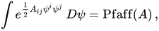
where A is an antisymmetric matrix, ψ is a collection of Grassmann variables, and the ⁠1/2⁠ is to prevent double-counting (since ψⁱψ^j = −ψ^jψⁱ).

In matrix notation, where ψ and η are Grassmann-valued row vectors, η and ψ are Grassmann-valued column vectors, and M is a real-valued matrix:

${\displaystyle Z=\int e^{\overline{\psi }M\psi +\overline{\eta }\psi +\overline{\psi }\eta }D\overline{\psi }D\psi =\int e^{\left(\overline{\psi }+\overline{\eta }{M}^{-1}\right)M\left(\psi +M^{-1}\eta \right)-\overline{\eta }{M}^{-1}\eta }D\overline{\psi }D\psi =\mathrm{D}\mathrm{e}\mathrm{t}(M)e^{-\overline{\eta }{M}^{-1}\eta },}$

where the last equality is a consequence of the translation invariance of the Grassmann integral. The Grassmann variables η are external sources for ψ, and differentiating with respect to η pulls down factors of ψ.

${\displaystyle ⟨\overline{\psi }\psi ⟩=\frac{1}{Z}\frac{\mathrm{\partial }}{\mathrm{\partial }\eta }\frac{\mathrm{\partial }}{\mathrm{\partial }\overline{\eta }}Z{|}_{\eta =\overline{\eta }=0}=M^{-1}}$

again, in a schematic matrix notation. The meaning of the formula above is that the derivative with respect to the appropriate component of η and η gives the matrix element of M⁻¹. This is exactly analogous to the bosonic path integration formula for a Gaussian integral of a complex bosonic field:

${\displaystyle \int e^{{\varphi }^{\ast }M\varphi +h^{\ast }\varphi +{\varphi }^{\ast }h}D{\varphi }^{\ast }D\varphi =\frac{e^{h^{\ast }{M}^{-1}h}}{\mathrm{D}\mathrm{e}\mathrm{t}(M)}}$

${\displaystyle ⟨{\varphi }^{\ast }\varphi ⟩=\frac{1}{Z}\frac{\mathrm{\partial }}{\mathrm{\partial }h}\frac{\mathrm{\partial }}{\mathrm{\partial }{h}^{\ast }}Z{|}_{h=h^{\ast }=0}=M^{-1}.}$

So that the propagator is the inverse of the matrix in the quadratic part of the action in both the Bose and Fermi case.

For real Grassmann fields, for Majorana fermions, the path integral is a Pfaffian times a source quadratic form, and the formulas give the square root of the determinant, just as they do for real Bosonic fields. The propagator is still the inverse of the quadratic part.

The free Dirac Lagrangian:

${\displaystyle \int \overline{\psi }\left({\gamma }^{\mu }{\mathrm{\partial }}_{\mu }-m\right)\psi }$

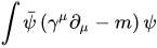
formally gives the equations of motion and the anticommutation relations of the Dirac field, just as the Klein Gordon Lagrangian in an ordinary path integral gives the equations of motion and commutation relations of the scalar field. By using the spatial Fourier transform of the Dirac field as a new basis for the Grassmann algebra, the quadratic part of the Dirac action becomes simple to invert:

${\displaystyle S={\int }_k\overline{\psi }\left(i{\gamma }^{\mu }{k}_{\mu }-m\right)\psi .}$

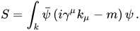
The propagator is the inverse of the matrix M linking ψ(k) and ψ(k), since different values of k do not mix together.

${\displaystyle ⟨\overline{\psi }(k^{\prime })\psi (k)⟩=\delta (k+k^{\prime })\frac{1}{\gamma \cdot k-m}=\delta (k+k^{\prime })\frac{\gamma \cdot k+m}{k^2-m^2}}$

The analog of Wick's theorem matches ψ and ψ in pairs:

${\displaystyle ⟨\overline{\psi }(k_1)\overline{\psi }(k_2)\cdots \overline{\psi }(k_n)\psi (k_1^{\prime })\cdots \psi (k_n)⟩=\sum _{\mathrm{p}\mathrm{a}\mathrm{i}\mathrm{r}\mathrm{i}\mathrm{n}\mathrm{g}\mathrm{s}}(-1{)}^S\prod _{\mathrm{p}\mathrm{a}\mathrm{i}\mathrm{r}\mathrm{s}i,j}\delta \left(k_i-k_j\right)\frac{1}{\gamma \cdot k_i-m}}$

where S is the sign of the permutation that reorders the sequence of ψ and ψ to put the ones that are paired up to make the delta-functions next to each other, with the ψ coming right before the ψ. Since a ψ, ψ pair is a commuting element of the Grassmann algebra, it does not matter what order the pairs are in. If more than one ψ, ψ pair have the same k, the integral is zero, and it is easy to check that the sum over pairings gives zero in this case (there are always an even number of them). This is the Grassmann analog of the higher Gaussian moments that completed the Bosonic Wick's theorem earlier.

The rules for spin-⁠1/2⁠ Dirac particles are as follows: The propagator is the inverse of the Dirac operator, the lines have arrows just as for a complex scalar field, and the diagram acquires an overall factor of −1 for each closed Fermi loop. If there are an odd number of Fermi loops, the diagram changes sign. Historically, the −1 rule was very difficult for Feynman to discover. He discovered it after a long process of trial and error, since he lacked a proper theory of Grassmann integration.

The rule follows from the observation that the number of Fermi lines at a vertex is always even. Each term in the Lagrangian must always be Bosonic. A Fermi loop is counted by following Fermionic lines until one comes back to the starting point, then removing those lines from the diagram. Repeating this process eventually erases all the Fermionic lines: this is the Euler algorithm to 2-color a graph, which works whenever each vertex has even degree. The number of steps in the Euler algorithm is only equal to the number of independent Fermionic homology cycles in the common special case that all terms in the Lagrangian are exactly quadratic in the Fermi fields, so that each vertex has exactly two Fermionic lines. When there are four-Fermi interactions (like in the Fermi effective theory of the weak nuclear interactions) there are more k-integrals than Fermi loops. In this case, the counting rule should apply the Euler algorithm by pairing up the Fermi lines at each vertex into pairs that together form a bosonic factor of the term in the Lagrangian, and when entering a vertex by one line, the algorithm should always leave with the partner line.

To clarify and prove the rule, consider a Feynman diagram formed from vertices, terms in the Lagrangian, with Fermion fields. The full term is Bosonic, it is a commuting element of the Grassmann algebra, so the order in which the vertices appear is not important. The Fermi lines are linked into loops, and when traversing the loop, one can reorder the vertex terms one after the other as one goes around without any sign cost. The exception is when you return to the starting point, and the final half-line must be joined with the unlinked first half-line. This requires one permutation to move the last ψ to go in front of the first ψ, and this gives the sign.

This rule is the only visible effect of the exclusion principle in internal lines. When there are external lines, the amplitudes are antisymmetric when two Fermi insertions for identical particles are interchanged. This is automatic in the source formalism, because the sources for Fermi fields are themselves Grassmann valued.

Spin 1: photons

The naive propagator for photons is infinite, since the Lagrangian for the A-field is:

${\displaystyle S=\int \frac{1}{4}{F}^{\mu \nu }{F}_{\mu \nu }=\int -\frac{1}{2}\left({\mathrm{\partial }}^{\mu }{A}_{\nu }{\mathrm{\partial }}_{\mu }{A}^{\nu }-{\mathrm{\partial }}^{\mu }{A}_{\mu }{\mathrm{\partial }}_{\nu }{A}^{\nu }\right).}$

The quadratic form defining the propagator is non-invertible. The reason is the gauge invariance of the field; adding a gradient to A does not change the physics.

To fix this problem, one needs to fix a gauge. The most convenient way is to demand that the divergence of A is some function f, whose value is random from point to point. It does no harm to integrate over the values of f, since it only determines the choice of gauge. This procedure inserts the following factor into the path integral for A:

${\displaystyle \int \delta \left({\mathrm{\partial }}_{\mu }{A}^{\mu }-f\right)e^{-\frac{f^2}{2}}Df.}$

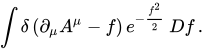
The first factor, the delta function, fixes the gauge. The second factor sums over different values of f that are inequivalent gauge fixings. This is simply

${\displaystyle e^{-\frac{{\left({\mathrm{\partial }}_{\mu }{A}_{\mu }\right)}^2}{2}}.}$

The additional contribution from gauge-fixing cancels the second half of the free Lagrangian, giving the Feynman Lagrangian:

${\displaystyle S=\int {\mathrm{\partial }}^{\mu }{A}^{\nu }{\mathrm{\partial }}_{\mu }{A}_{\nu }}$

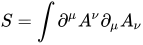
which is just like four independent free scalar fields, one for each component of A. The Feynman propagator is:

${\displaystyle ⟨A_{\mu }(k)A_{\nu }(k^{\prime })⟩=\delta \left(k+k^{\prime }\right)\frac{g_{\mu \nu }}{k^2}.}$

The one difference is that the sign of one propagator is wrong in the Lorentz case: the timelike component has an opposite sign propagator. This means that these particle states have negative norm—they are not physical states. In the case of photons, it is easy to show by diagram methods that these states are not physical—their contribution cancels with longitudinal photons to only leave two physical photon polarization contributions for any value of k.

If the averaging over f is done with a coefficient different from ⁠1/2⁠, the two terms do not cancel completely. This gives a covariant Lagrangian with a coefficient ${\displaystyle \lambda }$, which does not affect anything:

${\displaystyle S=\int \frac{1}{2}\left({\mathrm{\partial }}^{\mu }{A}^{\nu }{\mathrm{\partial }}_{\mu }{A}_{\nu }-\lambda {\left({\mathrm{\partial }}_{\mu }{A}^{\mu }\right)}^2\right)}$

and the covariant propagator for QED is:

${\displaystyle ⟨A_{\mu }(k)A_{\nu }(k^{\prime })⟩=\delta \left(k+k^{\prime }\right)\frac{g_{\mu \nu }-\lambda \frac{k_{\mu }{k}_{\nu }}{k^2}}{k^2}.}$

Spin 1: non-Abelian ghosts

To find the Feynman rules for non-Abelian gauge fields, the procedure that performs the gauge fixing must be carefully corrected to account for a change of variables in the path-integral.

The gauge fixing factor has an extra determinant from popping the delta function:

${\displaystyle \delta \left({\mathrm{\partial }}_{\mu }{A}_{\mu }-f\right)e^{-\frac{f^2}{2}}detM}$

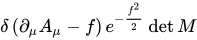
To find the form of the determinant, consider first a simple two-dimensional integral of a function f that depends only on r, not on the angle θ. Inserting an integral over θ:

${\displaystyle \int f(r)dxdy=\int f(r)\int d\theta \delta (y)\left|\frac{dy}{d\theta }\right|dxdy}$

The derivative-factor ensures that popping the delta function in θ removes the integral. Exchanging the order of integration,

${\displaystyle \int f(r)dxdy=\int d\theta \int f(r)\delta (y)\left|\frac{dy}{d\theta }\right|dxdy}$

but now the delta-function can be popped in y,

${\displaystyle \int f(r)dxdy=\int d{\theta }_0\int f(x)\left|\frac{dy}{d\theta }\right|dx.}$

The integral over θ just gives an overall factor of 2π, while the rate of change of y with a change in θ is just x, so this exercise reproduces the standard formula for polar integration of a radial function:

${\displaystyle \int f(r)dxdy=2\pi \int f(x)xdx}$

In the path-integral for a nonabelian gauge field, the analogous manipulation is:

${\displaystyle \int DA\int \delta (F(A))det\left(\frac{\mathrm{\partial }F}{\mathrm{\partial }G}\right)DG{e}^{iS}=\int DG\int \delta (F(A))det\left(\frac{\mathrm{\partial }F}{\mathrm{\partial }G}\right)e^{iS}}$

The factor in front is the volume of the gauge group, and it contributes a constant, which can be discarded. The remaining integral is over the gauge fixed action.

${\displaystyle \int det\left(\frac{\mathrm{\partial }F}{\mathrm{\partial }G}\right)e^{i{S}_{GF}}DA}$

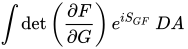
To get a covariant gauge, the gauge fixing condition is the same as in the Abelian case:

${\displaystyle {\mathrm{\partial }}_{\mu }{A}^{\mu }=f,}$

Whose variation under an infinitesimal gauge transformation is given by:

${\displaystyle {\mathrm{\partial }}_{\mu }{D}_{\mu }\alpha ,}$

where α is the adjoint valued element of the Lie algebra at every point that performs the infinitesimal gauge transformation. This adds the Faddeev Popov determinant to the action:

${\displaystyle det\left({\mathrm{\partial }}_{\mu }{D}_{\mu }\right)}$

which can be rewritten as a Grassmann integral by introducing ghost fields:

${\displaystyle \int e^{\overline{\eta }{\mathrm{\partial }}_{\mu }{D}^{\mu }\eta }D\overline{\eta }D\eta }$

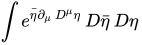
The determinant is independent of f, so the path-integral over f can give the Feynman propagator (or a covariant propagator) by choosing the measure for f as in the abelian case. The full gauge fixed action is then the Yang Mills action in Feynman gauge with an additional ghost action:

${\displaystyle S=\int \mathrm{Tr}{\mathrm{\partial }}_{\mu }{A}_{\nu }{\mathrm{\partial }}^{\mu }{A}^{\nu }+f_{jk}^i{\mathrm{\partial }}^{\nu }{A}_i^{\mu }{A}_{\mu }^j{A}_{\nu }^k+f_{jr}^i{f}_{kl}^r{A}_i{A}_j{A}^k{A}^l+\mathrm{Tr}{\mathrm{\partial }}_{\mu }\overline{\eta }{\mathrm{\partial }}^{\mu }\eta +\overline{\eta }{A}_j\eta }$

The diagrams are derived from this action. The propagator for the spin-1 fields has the usual Feynman form. There are vertices of degree 3 with momentum factors whose couplings are the structure constants, and vertices of degree 4 whose couplings are products of structure constants. There are additional ghost loops, which cancel out timelike and longitudinal states in A loops.

In the Abelian case, the determinant for covariant gauges does not depend on A, so the ghosts do not contribute to the connected diagrams.

Particle-path representation

Feynman diagrams were originally discovered by Feynman, by trial and error, as a way to represent the contribution to the S-matrix from different classes of particle trajectories.

Schwinger representation

The Euclidean scalar propagator has a suggestive representation:

${\displaystyle \frac{1}{p^2+m^2}={\int }_0^{\mathrm{\infty }}{e}^{-\tau \left(p^2+m^2\right)}d\tau }$

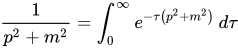
The meaning of this identity (which is an elementary integration) is made clearer by Fourier transforming to real space.

${\displaystyle \mathrm{\Delta }(x)={\int }_0^{\mathrm{\infty }}d\tau e^{-m^2\tau }\frac{1}{(4\pi \tau {)}^{d/2}}{e}^{\frac{-x^2}{4\tau }}}$

The contribution at any one value of τ to the propagator is a Gaussian of width ̀̀√τ. The total propagation function from 0 to x is a weighted sum over all proper times τ of a normalized Gaussian, the probability of ending up at x after a random walk of time τ.

The path-integral representation for the propagator is then:

${\displaystyle \mathrm{\Delta }(x)={\int }_0^{\mathrm{\infty }}d\tau \int DX{e}^{-\underset{0}{\overset{\tau }{\int }}\left(\frac{{\dot{x}}^2}{2}+m^2\right)d{\tau }^{\prime }}}$

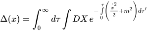
which is a path-integral rewrite of the Schwinger representation.

The Schwinger representation is both useful for making manifest the particle aspect of the propagator, and for symmetrizing denominators of loop diagrams.

Combining denominators

The Schwinger representation has an immediate practical application to loop diagrams. For example, for the diagram in the φ⁴ theory formed by joining two xs together in two half-lines, and making the remaining lines external, the integral over the internal propagators in the loop is:

${\displaystyle {\int }_k\frac{1}{k^2+m^2}\frac{1}{(k+p{)}^2+m^2}.}$

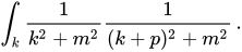
Here one line carries momentum k and the other k + p. The asymmetry can be fixed by putting everything in the Schwinger representation.

${\displaystyle {\int }_{t,t^{\prime }}{e}^{-t(k^2+m^2)-t^{\prime }\left((k+p{)}^2+m^2\right)}dtd{t}^{\prime }.}$

Now the exponent mostly depends on t + t′,

${\displaystyle {\int }_{t,t^{\prime }}{e}^{-(t+t^{\prime })(k^2+m^2)-t^{\prime }2p\cdot k-t^{\prime }{p}^2},}$

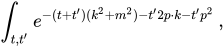
except for the asymmetrical little bit. Defining the variable u = t + t′ and v = ⁠t′/u⁠, the variable u goes from 0 to ∞, while v goes from 0 to 1. The variable u is the total proper time for the loop, while v parametrizes the fraction of the proper time on the top of the loop versus the bottom.

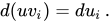
The Jacobian for this transformation of variables is easy to work out from the identities:

${\displaystyle d(uv)=d{t}^{\prime }du=dt+d{t}^{\prime },}$

and "wedging" gives

${\displaystyle udu\wedge dv=dt\wedge d{t}^{\prime }}$.

This allows the u integral to be evaluated explicitly:

${\displaystyle {\int }_{u,v}u{e}^{-u\left(k^2+m^2+v2p\cdot k+v{p}^2\right)}=\int \frac{1}{{\left(k^2+m^2+v2p\cdot k-v{p}^2\right)}^2}dv}$

leaving only the v-integral. This method, invented by Schwinger but usually attributed to Feynman, is called combining denominator. Abstractly, it is the elementary identity:

${\displaystyle \frac{1}{AB}={\int }_0^1\frac{1}{(vA+(1-v)B{)}^2}dv}$

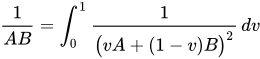
But this form does not provide the physical motivation for introducing v; v is the proportion of proper time on one of the legs of the loop.

Once the denominators are combined, a shift in k to k′ = k + vp symmetrizes everything:

${\displaystyle {\int }_0^1\int \frac{1}{{\left(k^2+m^2+2vp\cdot k+v{p}^2\right)}^2}dkdv={\int }_0^1\int \frac{1}{{\left(k^{\prime 2}+m^2+v(1-v)p^2\right)}^2}d{k}^{\prime }dv}$

This form shows that the moment that p² is more negative than four times the mass of the particle in the loop, which happens in a physical region of Lorentz space, the integral has a cut. This is exactly when the external momentum can create physical particles.

When the loop has more vertices, there are more denominators to combine:

${\displaystyle \int dk\frac{1}{k^2+m^2}\frac{1}{(k+p_1{)}^2+m^2}\cdots \frac{1}{(k+p_n{)}^2+m^2}}$

The general rule follows from the Schwinger prescription for n + 1 denominators:

${\displaystyle \frac{1}{D_0{D}_1\cdots D_n}={\int }_0^{\mathrm{\infty }}\cdots {\int }_0^{\mathrm{\infty }}{e}^{-u_0{D}_0\cdots -u_n{D}_n}d{u}_0\cdots d{u}_n.}$

The integral over the Schwinger parameters u_i can be split up as before into an integral over the total proper time u = u₀ + u₁ ... + u_n and an integral over the fraction of the proper time in all but the first segment of the loop v_i = ⁠u_i/u⁠ for i ∈ {1,2,...,n}. The v_i are positive and add up to less than 1, so that the v integral is over an n-dimensional simplex.

The Jacobian for the coordinate transformation can be worked out as before:

${\displaystyle du=d{u}_0+d{u}_1\cdots +d{u}_n}$

${\displaystyle d(u{v}_i)=d{u}_i.}$

Wedging all these equations together, one obtains

${\displaystyle u^{n}du\wedge d{v}_1\wedge d{v}_2\cdots \wedge d{v}_n=d{u}_0\wedge d{u}_1\cdots \wedge d{u}_n.}$

This gives the integral:

${\displaystyle {\int }_0^{\mathrm{\infty }}{\int }_{\mathrm{s}\mathrm{i}\mathrm{m}\mathrm{p}\mathrm{l}\mathrm{e}\mathrm{x}}{u}^n{e}^{-u\left(v_0{D}_0+v_1{D}_1+v_2{D}_2\cdots +v_n{D}_n\right)}d{v}_1\cdots d{v}_{n}du,}$

where the simplex is the region defined by the conditions

${\displaystyle v_i>0\text{and}\sum _{i=1}^n{v}_i<1}$

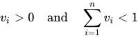
as well as

${\displaystyle v_0=1-\sum _{i=1}^n{v}_i.}$

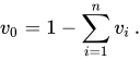
Performing the u integral gives the general prescription for combining denominators:

${\displaystyle \frac{1}{D_0\cdots D_n}=n!{\int }_{\mathrm{s}\mathrm{i}\mathrm{m}\mathrm{p}\mathrm{l}\mathrm{e}\mathrm{x}}\frac{1}{{\left(v_0{D}_0+v_1{D}_1\cdots +v_n{D}_n\right)}^{n+1}}d{v}_{1}d{v}_2\cdots d{v}_n}$

Since the numerator of the integrand is not involved, the same prescription works for any loop, no matter what the spins are carried by the legs. The interpretation of the parameters v_i is that they are the fraction of the total proper time spent on each leg.

Scattering

The correlation functions of a quantum field theory describe the scattering of particles. The definition of "particle" in relativistic field theory is not self-evident, because if you try to determine the position so that the uncertainty is less than the compton wavelength, the uncertainty in energy is large enough to produce more particles and antiparticles of the same type from the vacuum. This means that the notion of a single-particle state is to some extent incompatible with the notion of an object localized in space.

In the 1930s, Wigner gave a mathematical definition for single-particle states: they are a collection of states that form an irreducible representation of the Poincaré group. Single particle states describe an object with a finite mass, a well defined momentum, and a spin. This definition is fine for protons and neutrons, electrons and photons, but it excludes quarks, which are permanently confined, so the modern point of view is more accommodating: a particle is anything whose interaction can be described in terms of Feynman diagrams, which have an interpretation as a sum over particle trajectories.

A field operator can act to produce a one-particle state from the vacuum, which means that the field operator φ(x) produces a superposition of Wigner particle states. In the free field theory, the field produces one particle states only. But when there are interactions, the field operator can also produce 3-particle, 5-particle (if there is no +/− symmetry also 2, 4, 6 particle) states too. To compute the scattering amplitude for single particle states only requires a careful limit, sending the fields to infinity and integrating over space to get rid of the higher-order corrections.

The relation between scattering and correlation functions is the LSZ-theorem: The scattering amplitude for n particles to go to m particles in a scattering event is the given by the sum of the Feynman diagrams that go into the correlation function for n + m field insertions, leaving out the propagators for the external legs.

For example, for the λφ⁴ interaction of the previous section, the order λ contribution to the (Lorentz) correlation function is:

${\displaystyle ⟨\varphi (k_1)\varphi (k_2)\varphi (k_3)\varphi (k_4)⟩=\frac{i}{k_1^2}\frac{i}{k_2^2}\frac{i}{k_3^2}\frac{i}{k_4^2}i\lambda }$

Stripping off the external propagators, that is, removing the factors of ⁠i/k²⁠, gives the invariant scattering amplitude M:

${\displaystyle M=i\lambda }$

which is a constant, independent of the incoming and outgoing momentum. The interpretation of the scattering amplitude is that the sum of |M|² over all possible final states is the probability for the scattering event. The normalization of the single-particle states must be chosen carefully, however, to ensure that M is a relativistic invariant.

Non-relativistic single particle states are labeled by the momentum k, and they are chosen to have the same norm at every value of k. This is because the nonrelativistic unit operator on single particle states is:

${\displaystyle \int dk|k⟩⟨k|.}$

In relativity, the integral over the k-states for a particle of mass m integrates over a hyperbola in E,k space defined by the energy–momentum relation:

${\displaystyle E^2-k^2=m^2.}$

If the integral weighs each k point equally, the measure is not Lorentz-invariant. The invariant measure integrates over all values of k and E, restricting to the hyperbola with a Lorentz-invariant delta function:

${\displaystyle \int \delta (E^2-k^2-m^2)|E,k⟩⟨E,k|dEdk=\int \frac{dk}{2E}|k⟩⟨k|.}$

So the normalized k-states are different from the relativistically normalized k-states by a factor of

${\displaystyle \sqrt{E}={\left(k^2-m^2\right)}^{\frac{1}{4}}.}$

The invariant amplitude M is then the probability amplitude for relativistically normalized incoming states to become relativistically normalized outgoing states.

For nonrelativistic values of k, the relativistic normalization is the same as the nonrelativistic normalization (up to a constant factor ${\displaystyle \sqrt{m}}$). In this limit, the φ⁴ invariant scattering amplitude is still constant. The particles created by the field φ scatter in all directions with equal amplitude.

The nonrelativistic potential, which scatters in all directions with an equal amplitude (in the Born approximation), is one whose Fourier transform is constant—a delta-function potential. The lowest order scattering of the theory reveals the non-relativistic interpretation of this theory—it describes a collection of particles with a delta-function repulsion. Two such particles have an aversion to occupying the same point at the same time.

Nonperturbative effects

Thinking of Feynman diagrams as a perturbation series, nonperturbative effects like tunneling do not show up, because any effect that goes to zero faster than any polynomial does not affect the Taylor series. Even bound states are absent, since at any finite order particles are only exchanged a finite number of times, and to make a bound state, the binding force must last forever.

But this point of view is misleading, because the diagrams not only describe scattering, but they also are a representation of the short-distance field theory correlations. They encode not only asymptotic processes like particle scattering, they also describe the multiplication rules for fields, the operator product expansion. Nonperturbative tunneling processes involve field configurations that on average get big when the coupling constant gets small, but each configuration is a coherent superposition of particles whose local interactions are described by Feynman diagrams. When the coupling is small, these become collective processes that involve large numbers of particles, but where the interactions between each of the particles is simple. (The perturbation series of any interacting quantum field theory has zero radius of convergence, complicating the limit of the infinite series of diagrams needed (in the limit of vanishing coupling) to describe such field configurations.)

This means that nonperturbative effects show up asymptotically in resummations of infinite classes of diagrams, and these diagrams can be locally simple. The graphs determine the local equations of motion, while the allowed large-scale configurations describe non-perturbative physics. But because Feynman propagators are nonlocal in time, translating a field process to a coherent particle language is not completely intuitive, and has only been explicitly worked out in certain special cases. In the case of nonrelativistic bound states, the Bethe–Salpeter equation describes the class of diagrams to include to describe a relativistic atom. For quantum chromodynamics, the Shifman–Vainshtein–Zakharov sum rules describe non-perturbatively excited long-wavelength field modes in particle language, but only in a phenomenological way.

The number of Feynman diagrams at high orders of perturbation theory is very large, because there are as many diagrams as there are graphs with a given number of nodes. Nonperturbative effects leave a signature on the way in which the number of diagrams and resummations diverge at high order. It is only because non-perturbative effects appear in hidden form in diagrams that it was possible to analyze nonperturbative effects in string theory, where in many cases a Feynman description is the only one available.

In popular culture

• The use of the above diagram of the virtual particle producing a quark–antiquark pair was featured in the television sit-com The Big Bang Theory, in the episode "The Bat Jar Conjecture".
• PhD Comics of January 11, 2012, shows Feynman diagrams that visualize and describe quantum academic interactions, i.e. the paths followed by Ph.D. students when interacting with their advisors.
• Vacuum Diagrams, a science fiction story by Stephen Baxter, features the titular vacuum diagram, a specific type of Feynman diagram.
• Feynman and his wife, Gweneth Howarth, bought a Dodge Tradesman Maxivan in 1975, and had it painted with Feynman diagrams. The van is currently owned by video game designer and physicist Seamus Blackley. Qantum was the license plate ID.

Evidence-based medicine

From Wikipedia, the free encyclopedia

https://en.wikipedia.org/wiki/Evidence-based_medicine 

Evidence-based medicine (EBM), sometimes known within healthcare as evidence-based practice (EBP), is "the conscientious, explicit and judicious use of current best evidence in making decisions about the care of individual patients. It means integrating individual clinical expertise with the best available external clinical evidence from systematic research." The aim of EBM is to integrate the experience of the clinician, the values of the patient, and the best available scientific information to guide decision-making about clinical management. The term was originally used to describe an approach to teaching the practice of medicine and improving decisions by individual physicians about individual patients.

The EBM Pyramid is a tool that helps in visualizing the hierarchy of evidence in medicine, from least authoritative, like expert opinions, to most authoritative, like systematic reviews.

Adoption of evidence-based medicine is necessary in a human rights-based approach to public health and a precondition for accessing the right to health.

Background, history, and definition

Medicine has a long history of scientific inquiry into the prevention, diagnosis, and treatment of human disease. In the 11th century AD, Avicenna, a Persian physician and philosopher, developed an approach to EBM that was mostly similar to current ideas and practises.

The concept of a controlled clinical trial was first described in 1662 by Jan Baptist van Helmont in reference to the practice of bloodletting. Wrote Van Helmont:

Let us take out of the Hospitals, out of the Camps, or from elsewhere, 200, or 500 poor People, that have fevers or Pleuritis. Let us divide them in Halfes, let us cast lots, that one halfe of them may fall to my share, and the others to yours; I will cure them without blood-letting and sensible evacuation; but you do, as ye know ... we shall see how many Funerals both of us shall have...

The first published report describing the conduct and results of a controlled clinical trial was by James Lind, a Scottish naval surgeon who conducted research on scurvy during his time aboard HMS Salisbury in the Channel Fleet, while patrolling the Bay of Biscay. Lind divided the sailors participating in his experiment into six groups, so that the effects of various treatments could be fairly compared. Lind found improvement in symptoms and signs of scurvy among the group of men treated with lemons or oranges. He published a treatise describing the results of this experiment in 1753.

An early critique of statistical methods in medicine was published in 1835, in Comtes Rendus de l'Académie des Sciences, Paris, by a man referred to as "Mr Civiale".

In 1990, Gordon Guyatt, then a young internal medicine residency coordinator at McMaster University, introduced a teaching method he initially termed "Scientific Medicine." This approach emphasized applying critical appraisal techniques directly to bedside clinical decision-making, building on the work of his mentor, David Sackett. However, the concept met resistance from colleagues, as it implied that existing clinical practices lacked scientific rigor, even though this was likely true. To address this, Guyatt rebranded the approach as "Evidence-Based Medicine", a term first formally introduced in a 1991 editorial in the ACP Journal Club. Although the name was coined in 1991, it took several years after and a concerted efforts of many other teams to define the foundations of this method.

Although more popular in medicine, the concept of "evidence-based" is spreading to other disciplines, such as the humanities, and to languages other than English, albeit at a slower pace.

Clinical decision-making

Alvan Feinstein's publication of Clinical Judgment in 1967 focused attention on the role of clinical reasoning and identified biases that can affect it. In 1972, Archie Cochrane published Effectiveness and Efficiency, which described the lack of controlled trials supporting many practices that had previously been assumed to be effective. In 1973, John Wennberg began to document wide variations in how physicians practiced. Through the 1980s, David M. Eddy described errors in clinical reasoning and gaps in evidence. In the mid-1980s, Alvin Feinstein, David Sackett and others published textbooks on clinical epidemiology, which translated epidemiological methods to physician decision-making. Toward the end of the 1980s, a group at RAND showed that large proportions of procedures performed by physicians were considered inappropriate even by the standards of their own experts.

Evidence-based guidelines and policies

Main article: Medical guideline

David M. Eddy first began to use the term 'evidence-based' in 1987 in workshops and a manual commissioned by the Council of Medical Specialty Societies to teach formal methods for designing clinical practice guidelines. The manual was eventually published by the American College of Physicians. Eddy first published the term 'evidence-based' in March 1990, in an article in the Journal of the American Medical Association (JAMA) that laid out the principles of evidence-based guidelines and population-level policies, which Eddy described as "explicitly describing the available evidence that pertains to a policy and tying the policy to evidence instead of standard-of-care practices or the beliefs of experts. The pertinent evidence must be identified, described, and analyzed. The policymakers must determine whether the policy is justified by the evidence. A rationale must be written." He discussed evidence-based policies in several other papers published in JAMA in the spring of 1990. Those papers were part of a series of 28 published in JAMA between 1990 and 1997 on formal methods for designing population-level guidelines and policies.

Medical education

The term 'evidence-based medicine' was introduced slightly later, in the context of medical education. In the autumn of 1990, Gordon Guyatt used it in an unpublished description of a program at McMaster University for prospective or new medical students. Guyatt and others first published the term two years later (1992) to describe a new approach to teaching the practice of medicine.

In 1996, David Sackett and colleagues clarified the definition of this tributary of evidence-based medicine as "the conscientious, explicit and judicious use of current best evidence in making decisions about the care of individual patients. ... [It] means integrating individual clinical expertise with the best available external clinical evidence from systematic research." This branch of evidence-based medicine aims to make individual decision making more structured and objective by better reflecting the evidence from research. Population-based data are applied to the care of an individual patient, while respecting the fact that practitioners have clinical expertise reflected in effective and efficient diagnosis and thoughtful identification and compassionate use of individual patients' predicaments, rights, and preferences.

Between 1993 and 2000, the Evidence-Based Medicine Working Group at McMaster University published the methods to a broad physician audience in a series of 25 "Users' Guides to the Medical Literature" in JAMA. In 1995 Rosenberg and Donald defined individual-level, evidence-based medicine as "the process of finding, appraising, and using contemporaneous research findings as the basis for medical decisions." In 2010, Greenhalgh used a definition that emphasized quantitative methods: "the use of mathematical estimates of the risk of benefit and harm, derived from high-quality research on population samples, to inform clinical decision-making in the diagnosis, investigation or management of individual patients."

The two original definitions highlight important differences in how evidence-based medicine is applied to populations versus individuals. When designing guidelines applied to large groups of people in settings with relatively little opportunity for modification by individual physicians, evidence-based policymaking emphasizes that good evidence should exist to document a test's or treatment's effectiveness. In the setting of individual decision-making, practitioners can be given greater latitude in how they interpret research and combine it with their clinical judgment. In 2005, Eddy offered an umbrella definition for the two branches of EBM: "Evidence-based medicine is a set of principles and methods intended to ensure that to the greatest extent possible, medical decisions, guidelines, and other types of policies are based on and consistent with good evidence of effectiveness and benefit."

Progress

In the area of evidence-based guidelines and policies, the explicit insistence on evidence of effectiveness was introduced by the American Cancer Society in 1980. The U.S. Preventive Services Task Force (USPSTF) began issuing guidelines for preventive interventions based on evidence-based principles in 1984. In 1985, the Blue Cross Blue Shield Association applied strict evidence-based criteria for covering new technologies. Beginning in 1987, specialty societies such as the American College of Physicians, and voluntary health organizations such as the American Heart Association, wrote many evidence-based guidelines. In 1991, Kaiser Permanente, a managed care organization in the US, began an evidence-based guidelines program. In 1991, Richard Smith wrote an editorial in the British Medical Journal and introduced the ideas of evidence-based policies in the UK. In 1993, the Cochrane Collaboration created a network of 13 countries to produce systematic reviews and guidelines. In 1997, the US Agency for Healthcare Research and Quality (AHRQ, then known as the Agency for Health Care Policy and Research, or AHCPR) established Evidence-based Practice Centers (EPCs) to produce evidence reports and technology assessments to support the development of guidelines. In the same year, a National Guideline Clearinghouse that followed the principles of evidence-based policies was created by AHRQ, the AMA, and the American Association of Health Plans (now America's Health Insurance Plans). In 1999, the National Institute for Clinical Excellence (NICE) was created in the UK to circulate evidence and guidance on treatments within the NHS.

In the area of medical education, medical schools in Canada, the US, the UK, Australia, and other countries now offer programs that teach evidence-based medicine. A 2009 study of UK programs found that more than half of UK medical schools offered some training in evidence-based medicine, although the methods and content varied considerably, and EBM teaching was restricted by lack of curriculum time, trained tutors and teaching materials. Many programs have been developed to help individual physicians gain better access to evidence. For example, UpToDate was created in the early 1990s. The Cochrane Collaboration began publishing evidence reviews in 1993. In 1995, BMJ Publishing Group launched Clinical Evidence, a 6-monthly periodical that provided brief summaries of the current state of evidence about important clinical questions for clinicians.

Current practice

By 2000, use of the term evidence-based had extended to other levels of the health care system. An example is evidence-based health services, which seek to increase the competence of health service decision makers and the practice of evidence-based medicine at the organizational or institutional level.

The multiple tributaries of evidence-based medicine share an emphasis on the importance of incorporating evidence from formal research in medical policies and decisions. However, because they differ on the extent to which they require good evidence of effectiveness before promoting a guideline or payment policy, a distinction is sometimes made between evidence-based medicine and science-based medicine, which also takes into account factors such as prior plausibility and compatibility with established science (as when medical organizations promote controversial treatments such as acupuncture). Differences also exist regarding the extent to which it is feasible to incorporate individual-level information in decisions. Thus, evidence-based guidelines and policies may not readily "hybridise" with experience-based practices orientated towards ethical clinical judgement, and can lead to contradictions, contest, and unintended crises. The most effective "knowledge leaders" (managers and clinical leaders) use a broad range of management knowledge in their decision making, rather than just formal evidence. Evidence-based guidelines may provide the basis for governmentality in health care, and consequently play a central role in the governance of contemporary health care systems.

Methods

Steps

The steps for designing explicit, evidence-based guidelines were described in the late 1980s: formulate the question (population, intervention, comparison intervention, outcomes, time horizon, setting); search the literature to identify studies that inform the question; interpret each study to determine precisely what it says about the question; if several studies address the question, synthesize their results (meta-analysis); summarize the evidence in evidence tables; compare the benefits, harms and costs in a balance sheet; draw a conclusion about the preferred practice; write the guideline; write the rationale for the guideline; have others review each of the previous steps; implement the guideline.

For the purposes of medical education and individual-level decision making, five steps of EBM in practice were described in 1992 and the experience of delegates attending the 2003 Conference of Evidence-Based Health Care Teachers and Developers was summarized into five steps and published in 2005. This five-step process can broadly be categorized as follows:

1. Translation of uncertainty to an answerable question; includes critical questioning, study design and levels of evidence
2. Systematic retrieval of the best evidence available
3. Critical appraisal of evidence for internal validity that can be broken down into aspects regarding:
   • Systematic errors as a result of selection bias, information bias and confounding
   • Quantitative aspects of diagnosis and treatment
   • The effect size and aspects regarding its precision
   • Clinical importance of results
   • External validity or generalizability
4. Application of results in practice
5. Evaluation of performance

Evidence reviews

Systematic reviews of published research studies are a major part of the evaluation of particular treatments. The Cochrane Collaboration is one of the best-known organisations that conducts systematic reviews. Like other producers of systematic reviews, it requires authors to provide a detailed study protocol as well as a reproducible plan of their literature search and evaluations of the evidence. After the best evidence is assessed, treatment is categorized as (1) likely to be beneficial, (2) likely to be harmful, or (3) without evidence to support either benefit or harm.

A 2007 analysis of 1,016 systematic reviews from all 50 Cochrane Collaboration Review Groups found that 44% of the reviews concluded that the intervention was likely to be beneficial, 7% concluded that the intervention was likely to be harmful, and 49% concluded that evidence did not support either benefit or harm. 96% recommended further research. In 2017, a study assessed the role of systematic reviews produced by Cochrane Collaboration to inform US private payers' policymaking; it showed that although the medical policy documents of major US private payers were informed by Cochrane systematic reviews, there was still scope to encourage the further use.

Assessing the quality of evidence

Main article: Levels of evidence

Evidence-based medicine categorizes different types of clinical evidence and rates or grades them according to the strength of their freedom from the various biases that beset medical research. For example, the strongest evidence for therapeutic interventions is provided by systematic review of randomized, well-blinded, placebo-controlled trials with allocation concealment and complete follow-up involving a homogeneous patient population and medical condition. In contrast, patient testimonials, case reports, and even expert opinion have little value as proof because of the placebo effect, the biases inherent in observation and reporting of cases, and difficulties in ascertaining who is an expert (however, some critics have argued that expert opinion "does not belong in the rankings of the quality of empirical evidence because it does not represent a form of empirical evidence" and continue that "expert opinion would seem to be a separate, complex type of knowledge that would not fit into hierarchies otherwise limited to empirical evidence alone.").

Several organizations have developed grading systems for assessing the quality of evidence. For example, in 1989 the U.S. Preventive Services Task Force (USPSTF) put forth the following system:

• Level I: Evidence obtained from at least one properly designed randomized controlled trial.
• Level II-1: Evidence obtained from well-designed controlled trials without randomization.
• Level II-2: Evidence obtained from well-designed cohort studies or case-control studies, preferably from more than one center or research group.
• Level II-3: Evidence obtained from multiple time series designs with or without the intervention. Dramatic results in uncontrolled trials might also be regarded as this type of evidence.
• Level III: Opinions of respected authorities, based on clinical experience, descriptive studies, or reports of expert committees.

Another example are the Oxford CEBM Levels of Evidence published by the Centre for Evidence-Based Medicine. First released in September 2000, the Levels of Evidence provide a way to rank evidence for claims about prognosis, diagnosis, treatment benefits, treatment harms, and screening, which most grading schemes do not address. The original CEBM Levels were Evidence-Based On Call to make the process of finding evidence feasible and its results explicit. In 2011, an international team redesigned the Oxford CEBM Levels to make them more understandable and to take into account recent developments in evidence ranking schemes. The Oxford CEBM Levels of Evidence have been used by patients and clinicians, as well as by experts to develop clinical guidelines, such as recommendations for the optimal use of phototherapy and topical therapy in psoriasis and guidelines for the use of the BCLC staging system for diagnosing and monitoring hepatocellular carcinoma in Canada.

In 2000, a system was developed by the Grading of Recommendations Assessment, Development and Evaluation (GRADE) working group. The GRADE system takes into account more dimensions than just the quality of medical research. It requires users who are performing an assessment of the quality of evidence, usually as part of a systematic review, to consider the impact of different factors on their confidence in the results. Authors of GRADE tables assign one of four levels to evaluate the quality of evidence, on the basis of their confidence that the observed effect (a numeric value) is close to the true effect. The confidence value is based on judgments assigned in five different domains in a structured manner. The GRADE working group defines 'quality of evidence' and 'strength of recommendations' based on the quality as two different concepts that are commonly confused with each other.

Systematic reviews may include randomized controlled trials that have low risk of bias, or observational studies that have high risk of bias. In the case of randomized controlled trials, the quality of evidence is high but can be downgraded in five different domains.

• Risk of bias: A judgment made on the basis of the chance that bias in included studies has influenced the estimate of effect.
• Imprecision: A judgment made on the basis of the chance that the observed estimate of effect could change completely.
• Indirectness: A judgment made on the basis of the differences in characteristics of how the study was conducted and how the results are actually going to be applied.
• Inconsistency: A judgment made on the basis of the variability of results across the included studies.
• Publication bias: A judgment made on the basis of the question whether all the research evidence has been taken to account.

In the case of observational studies per GRADE, the quality of evidence starts off lower and may be upgraded in three domains in addition to being subject to downgrading.

• Large effect: Methodologically strong studies show that the observed effect is so large that the probability of it changing completely is less likely.
• Plausible confounding would change the effect: Despite the presence of a possible confounding factor that is expected to reduce the observed effect, the effect estimate still shows significant effect.
• Dose response gradient: The intervention used becomes more effective with increasing dose. This suggests that a further increase will likely bring about more effect.

Meaning of the levels of quality of evidence as per GRADE:

• High Quality Evidence: The authors are very confident that the presented estimate lies very close to the true value. In other words, the probability is very low that further research will completely change the presented conclusions.
• Moderate Quality Evidence: The authors are confident that the presented estimate lies close to the true value, but it is also possible that it may be substantially different. In other words, further research may completely change the conclusions.
• Low Quality Evidence: The authors are not confident in the effect estimate, and the true value may be substantially different. In other words, further research is likely to change the presented conclusions completely.
• Very Low Quality Evidence: The authors do not have any confidence in the estimate and it is likely that the true value is substantially different from it. In other words, new research will probably change the presented conclusions completely.

Categories of recommendations

In guidelines and other publications, recommendation for a clinical service is classified by the balance of risk versus benefit and the level of evidence on which this information is based. The U.S. Preventive Services Task Force uses the following system:

• Level A: Good scientific evidence suggests that the benefits of the clinical service substantially outweigh the potential risks. Clinicians should discuss the service with eligible patients.
• Level B: At least fair scientific evidence suggests that the benefits of the clinical service outweighs the potential risks. Clinicians should discuss the service with eligible patients.
• Level C: At least fair scientific evidence suggests that the clinical service provides benefits, but the balance between benefits and risks is too close for general recommendations. Clinicians need not offer it unless individual considerations apply.
• Level D: At least fair scientific evidence suggests that the risks of the clinical service outweigh potential benefits. Clinicians should not routinely offer the service to asymptomatic patients.
• Level I: Scientific evidence is lacking, of poor quality, or conflicting, such that the risk versus benefit balance cannot be assessed. Clinicians should help patients understand the uncertainty surrounding the clinical service.

GRADE guideline panelists may make strong or weak recommendations on the basis of further criteria. Some of the important criteria are the balance between desirable and undesirable effects (not considering cost), the quality of the evidence, values and preferences and costs (resource utilization).

Despite the differences between systems, the purposes are the same: to guide users of clinical research information on which studies are likely to be most valid. However, the individual studies still require careful critical appraisal.

Statistical measures

Evidence-based medicine attempts to express clinical benefits of tests and treatments using mathematical methods. Tools used by practitioners of evidence-based medicine include:

• Likelihood ratio
  Main article: Likelihood ratios in diagnostic testing
  The pre-test odds of a particular diagnosis, multiplied by the likelihood ratio, determines the post-test odds. (Odds can be calculated from, and then converted to, the [more familiar] probability.) This reflects Bayes' theorem. The differences in likelihood ratio between clinical tests can be used to prioritize clinical tests according to their usefulness in a given clinical situation.
• AUC-ROC The area under the receiver operating characteristic curve (AUC-ROC) reflects the relationship between sensitivity and specificity for a given test. High-quality tests will have an AUC-ROC approaching 1, and high-quality publications about clinical tests will provide information about the AUC-ROC. Cutoff values for positive and negative tests can influence specificity and sensitivity, but they do not affect AUC-ROC.
• Number needed to treat (NNT)/Number needed to harm (NNH). NNT and NNH are ways of expressing the effectiveness and safety, respectively, of interventions in a way that is clinically meaningful. NNT is the number of people who need to be treated in order to achieve the desired outcome (e.g. survival from cancer) in one patient. For example, if a treatment increases the chance of survival by 5%, then 20 people need to be treated in order for 1 additional patient to survive because of the treatment. The concept can also be applied to diagnostic tests. For example, if 1,339 women age 50–59 need to be invited for breast cancer screening over a ten-year period in order to prevent one woman from dying of breast cancer, then the NNT for being invited to breast cancer screening is 1339.

Quality of clinical trials

Evidence-based medicine attempts to objectively evaluate the quality of clinical research by critically assessing techniques reported by researchers in their publications.

• Trial design considerations: High-quality studies have clearly defined eligibility criteria and have minimal missing data.
• Generalizability considerations: Studies may only be applicable to narrowly defined patient populations and may not be generalizable to other clinical contexts.
• Follow-up: Sufficient time for defined outcomes to occur can influence the prospective study outcomes and the statistical power of a study to detect differences between a treatment and control arm.
• Power: A mathematical calculation can determine whether the number of patients is sufficient to detect a difference between treatment arms. A negative study may reflect a lack of benefit, or simply a lack of sufficient quantities of patients to detect a difference.

Limitations and criticism

There are a number of limitations and criticisms of evidence-based medicine. Two widely cited categorization schemes for the various published critiques of EBM include the three-fold division of Straus and McAlister ("limitations universal to the practice of medicine, limitations unique to evidence-based medicine and misperceptions of evidence-based-medicine") and the five-point categorization of Cohen, Stavri and Hersh (EBM is a poor philosophic basis for medicine, defines evidence too narrowly, is not evidence-based, is limited in usefulness when applied to individual patients, or reduces the autonomy of the doctor/patient relationship).

In no particular order, some published objections include:

• Research produced by EBM, such as from randomized controlled trials (RCTs), may not be relevant for all treatment situations. Research tends to focus on specific populations, but individual persons can vary substantially from population norms. Because certain population segments have been historically under-researched (due to reasons such as race, gender, age, and co-morbid diseases), evidence from RCTs may not be generalizable to those populations. Thus, EBM applies to groups of people, but this should not preclude clinicians from using their personal experience in deciding how to treat each patient. One author advises that "the knowledge gained from clinical research does not directly answer the primary clinical question of what is best for the patient at hand" and suggests that evidence-based medicine should not discount the value of clinical experience. Another author stated that "the practice of evidence-based medicine means integrating individual clinical expertise with the best available external clinical evidence from systematic research."
• Use of evidence-based guidelines often fits poorly for complex, multimorbid patients. This is because the guidelines are usually based on clinical studies focused on single diseases. In reality, the recommended treatments in such circumstances may interact unfavorably with each other and often lead to polypharmacy.
• The theoretical ideal of EBM (that every narrow clinical question, of which hundreds of thousands can exist, would be answered by meta-analysis and systematic reviews of multiple RCTs) faces the limitation that research (especially the RCTs themselves) is expensive; thus, in reality, for the foreseeable future, the demand for EBM will always be much higher than the supply, and the best humanity can do is to triage the application of scarce resources.
• Research can be influenced by biases such as political or belief bias, publication bias and conflict of interest in academic publishing. For example, studies with conflicts due to industry funding are more likely to favor their product. It has been argued that contemporary evidence based medicine is an illusion, since evidence based medicine has been corrupted by corporate interests, failed regulation, and commercialisation of academia.
• Systematic Reviews methodologies are capable of bias and abuse in respect of (i) choice of inclusion criteria (ii) choice of outcome measures, comparisons and analyses (iii) the subjectivity inevitable in Risk of Bias assessments, even when codified procedures and criteria are observed. An example of all these problems can be seen in a Cochrane Review.
• A lag exists between when the RCT is conducted and when its results are published.
• A lag exists between when results are published and when they are properly applied.
• Hypocognition (the absence of a simple, consolidated mental framework into which new information can be placed) can hinder the application of EBM.
• Values: while patient values are considered in the original definition of EBM, the importance of values is not commonly emphasized in EBM training, a potential problem under current study.

A 2018 study, "Why all randomised controlled trials produce biased results", assessed the 10 most cited RCTs and argued that trials face a wide range of biases and constraints, from trials only being able to study a small set of questions amenable to randomisation and generally only being able to assess the average treatment effect of a sample, to limitations in extrapolating results to another context, among many others outlined in the study.

Application of evidence in clinical settings

Despite the emphasis on evidence-based medicine, unsafe or ineffective medical practices continue to be applied, because of patient demand for tests or treatments, because of failure to access information about the evidence, or because of the rapid pace of change in the scientific evidence. For example, between 2003 and 2017, the evidence shifted on hundreds of medical practices, including whether hormone replacement therapy was safe, whether babies should be given certain vitamins, and whether antidepressant drugs are effective in people with Alzheimer's disease. Even when the evidence unequivocally shows that a treatment is either not safe or not effective, it may take many years for other treatments to be adopted.

There are many factors that contribute to lack of uptake or implementation of evidence-based recommendations. These include lack of awareness at the individual clinician or patient (micro) level, lack of institutional support at the organisation level (meso) level or higher at the policy (macro) level. In other cases, significant change can require a generation of physicians to retire or die and be replaced by physicians who were trained with more recent evidence.

Physicians may also reject evidence that conflicts with their anecdotal experience or because of cognitive biases – for example, a vivid memory of a rare but shocking outcome (the availability heuristic), such as a patient dying after refusing treatment. They may overtreat to "do something" or to address a patient's emotional needs. They may worry about malpractice charges based on a discrepancy between what the patient expects and what the evidence recommends. They may also overtreat or provide ineffective treatments because the treatment feels biologically plausible.

It is the responsibility of those developing clinical guidelines to include an implementation plan to facilitate uptake. The implementation process will include an implementation plan, analysis of the context, identifying barriers and facilitators and designing the strategies to address them.

Education

Training in evidence based medicine is offered across the continuum of medical education. Educational competencies have been created for the education of health care professionals.

The Berlin questionnaire and the Fresno Test are validated instruments for assessing the effectiveness of education in evidence-based medicine. These questionnaires have been used in diverse settings.

A Campbell systematic review that included 24 trials examined the effectiveness of e-learning in improving evidence-based health care knowledge and practice. It was found that e-learning, compared to no learning, improves evidence-based health care knowledge and skills but not attitudes and behaviour. No difference in outcomes is present when comparing e-learning with face-to-face learning. Combining e-learning and face-to-face learning (blended learning) has a positive impact on evidence-based knowledge, skills, attitude and behavior. As a form of e-learning, some medical school students engage in editing Wikipedia to increase their EBM skills, and some students construct EBM materials to develop their skills in communicating medical knowledge.

Naturalistic fallacy

From Wikipedia, the free encyclopedia

https://en.wikipedia.org/wiki/Naturalistic_fallacy

In metaethics, the naturalistic fallacy is the claim that it is possible to define good in terms of merely described entities, properties, or processes such as pleasant, desirable, or fitness. The term was introduced by British philosopher G. E. Moore in his 1903 book Principia Ethica.

Moore's naturalistic fallacy is closely related to the is–ought problem, which comes from David Hume's Treatise of Human Nature (1738–40); however, unlike Hume's view of the is–ought problem, Moore (and other proponents of ethical non-naturalism) did not consider the naturalistic fallacy to be at odds with moral realism.

Common uses

The is–ought problem

Main article: Is–ought problem

The term naturalistic fallacy is sometimes used to label the problematic inference of an ought from an is (the is–ought problem). Michael Ridge relevantly elaborates that "[t]he intuitive idea is that evaluative conclusions require at least one evaluative premise—purely factual premises about the naturalistic features of things do not entail or even support evaluative conclusions." This problematic inference usually takes the form of saying that if people generally do something (e.g., eat three times a day, smoke cigarettes, dress warmly in cold weather), then people ought to do that thing. The naturalistic fallacy occurs when the is–ought inference ("People eat three times a day, so it is morally good for people to eat three times a day") is justified by the claim that whatever practice exists is a natural one ("because eating three times a day is pleasant and desirable").

Bentham, in discussing the relations of law and morality, found that when people discuss problems and issues they talk about how they wish it would be, instead of how it actually is. This can be seen in discussions of natural law and positive law. Bentham criticized natural law theory because in his view it was an instance of the naturalistic fallacy, claiming that it described how things are rather than how they ought to be.

Moore's discussion

The title page of Principia Ethica

According to G. E. Moore's Principia Ethica, when philosophers try to define good reductively, in terms of natural properties like pleasant or desirable, they are committing the naturalistic fallacy:

... the assumption that because some quality or combination of qualities invariably and necessarily accompanies the quality of goodness, or is invariably and necessarily accompanied by it, or both, this quality or combination of qualities is identical with goodness. If, for example, it is believed that whatever is pleasant is and must be good, or that whatever is good is and must be pleasant, or both, it is committing the naturalistic fallacy to infer from this that goodness and pleasantness are one and the same quality. The naturalistic fallacy is the assumption that because the words 'good' and, say, 'pleasant' necessarily describe the same objects, they must attribute the same quality to them.

— Arthur N. Prior, Logic And The Basis Of Ethics

In defense of ethical non-naturalism against ethical naturalism, Moore's argument is concerned with the semantic and metaphysical underpinnings of ethics. Moore argues that good, in the sense of intrinsic value, is simply ineffable. It cannot be defined because it is not reducible to other properties, being "one of those innumerable objects of thought which are themselves incapable of definition, because they are the ultimate terms by reference to which whatever 'is' capable of definition must be defined".^[5] On the other hand, ethical naturalists eschew such principles in favor of a more empirically accessible analysis of what it means to be good: for example, in terms of pleasure in the context of hedonism.

That "pleased" does not mean "having the sensation of red", or anything else whatever, does not prevent us from understanding what it does mean. It is enough for us to know that "pleased" does mean "having the sensation of pleasure", and though pleasure is absolutely indefinable, though pleasure is pleasure and nothing else whatever, yet we feel no difficulty in saying that we are pleased. The reason is, of course, that when I say "I am pleased", I do not mean that "I" am the same thing as "having pleasure". And similarly no difficulty need be found in my saying that "pleasure is good" and yet not meaning that "pleasure" is the same thing as "good", that pleasure means good, and that good means pleasure. If I were to imagine that when I said "I am pleased", I meant that I was exactly the same thing as "pleased", I should not indeed call that a naturalistic fallacy, although it would be the same fallacy as I have called naturalistic with reference to Ethics.

— G. E. Moore, Principia Ethica § 12

In §7, Moore argues that a property is either a complex of simple properties, or else it is irreducibly simple. Complex properties can be defined in terms of their constituent parts but a simple property lacks parts. In addition to good and pleasure, Moore suggests that colour qualia are undefined: if one wants to understand yellow, one must see examples of it. It will do no good to read the dictionary and learn that yellow names the colour of egg yolks and ripe lemons, or that yellow names the primary colour between green and orange on the spectrum, or that the perception of yellow is stimulated by electromagnetic radiation with a wavelength of between 570 and 590 nanometers, because yellow is all that and more, by the open question argument.

Appeal to nature

Main article: Appeal to nature

Some people use the phrase, naturalistic fallacy or appeal to nature, in a different sense, to characterize inferences of the form "Something is natural; therefore, it is morally acceptable" or "This property is unnatural; therefore, this property is undesirable." Such inferences are common in discussions of medicine, homosexuality, environmentalism, and veganism.

The naturalistic fallacy is the idea that what is found in nature is good. It was the basis for social Darwinism, the belief that helping the poor and sick would get in the way of evolution, which depends on the survival of the fittest. Today, biologists denounce the naturalistic fallacy because they want to describe the natural world honestly, without people deriving morals about how we ought to behave (as in: If birds and beasts engage in adultery, infanticide, cannibalism, it must be OK).

— Steven Pinker

Criticism

See also: Is–ought problem § Responses

Bernard Williams called Moore's use of the term naturalistic fallacy a "spectacular misnomer", the matter in question being metaphysical, as opposed to rational.

Some philosophers reject the naturalistic fallacy or suggest solutions for the proposed is–ought problem.

Bound-up functions

Ralph McInerny suggests that ought is already bound up in is, insofar as the very nature of things have ends/goals within them. For example, a clock is a device used to keep time. When one understands the function of a clock, then a standard of evaluation is implicit in the very description of the clock, i.e., because it is a clock, it ought to keep the time. Thus, if one cannot pick a good clock from a bad clock, then one does not really know what a clock is. In like manner, if one cannot determine good human action from bad, then one does not really know what the human person is.

Irrationality of anti-naturalistic fallacy

The belief that naturalistic fallacy is inherently flawed has been criticized as lacking rational bases, and labelled anti-naturalistic fallacy. For instance, Alex Walter wrote:

"The naturalistic fallacy and Hume's 'law' are frequently appealed to for the purpose of drawing limits around the scope of scientific inquiry into ethics and morality. These two objections are shown to be without force."

That is because said beliefs implicitly assert that there is no connection between the facts and the norms (in particular, between the facts and the mental process that led to adoption of the norms). However, some philosophers argue that these connections are inevitable.

A very basic example is that if people view rescuing people as morally correct, this would shape their beliefs on what constitutes danger and what situations warrant intervention. For wider-ranging examples, if one believes that a certain ethnic group of humans have a population-level statistical hereditary predisposition to destroy civilization while the other person does not believe that such is the case, that difference in beliefs about factual matters will make the first person conclude that persecution of said ethnic group is an excusable "necessary evil" while the second person will conclude that it is a totally unjustifiable evil.

Similarly, if two people think it is evil to keep people working extremely hard in extreme poverty, they will draw different conclusions on de facto rights (as opposed to purely semantic rights) of property owners. The latter is dependent on whether they believe property owners are responsible for the aforementioned exploitation. One who accepts this premise would conclude that it is necessary to persecute property owners to mitigate exploitation. The one who does not, on the other hand, would conclude that the persecution is unnecessary and evil.

Inconsistent application

Some critics of the assumption that is-ought conclusions are fallacies point at observations of people who purport to consider such conclusions as fallacies do not do so consistently. Examples mentioned are that evolutionary psychologists who gripe about "the naturalistic fallacy" do make is-ought conclusions themselves when, for instance, alleging that the notion of the blank slate would lead to totalitarian social engineering or that certain views on sexuality would lead to attempts to convert homosexuals to heterosexuals. Critics point at this as a sign that charges of the naturalistic fallacy are inconsistent rhetorical tactics rather than detection of a fallacy.

Universally normative allegations of varied harm

A criticism of the concept of the naturalistic fallacy is that while "descriptive" statements (used here in the broad sense about statements that purport to be about facts regardless of whether they are true or false, used simply as opposed to normative statements) about specific differences in effects can be inverted depending on values (such as the statement "people X are predisposed to eating babies" being normative against group X only in the context of protecting children while the statement "individual or group X is predisposed to emit greenhouse gases" is normative against individual/group X only in the context of protecting the environment), the statement "individual/group X is predisposed to harm whatever values others have" is universally normative against individual/group X. This refers to individual/group X being "descriptively" alleged to detect what other entities capable of valuing are protecting and then destroying it without individual/group X having any values of its own. For example, in the context of one philosophy advocating child protection considering eating babies the worst evil and advocating industries that emit greenhouse gases to finance a safe short term environment for children while another philosophy considers long term damage to the environment the worst evil and advocates eating babies to reduce overpopulation and with it consumption that emits greenhouse gases, such an individual/group X could be alleged to advocate both eating babies and building autonomous industries to maximize greenhouse gas emissions, making the two otherwise enemy philosophies become allies against individual/group X as a "common enemy". The principle, that of allegations of an individual or group being predisposed to adapt their harm to damage any values including combined harm of apparently opposite values inevitably making normative implications regardless of which the specific values are, is argued to extend to any other situations with any other values as well due to the allegation being of the individual or group adapting their destruction to different values. This is mentioned as an example of at least one type of "descriptive" allegation being bound to make universally normative implications, as well as the allegation not being scientifically self-correcting due to individual or group X being alleged to manipulate others to support their alleged all-destructive agenda which dismisses any scientific criticism of the allegation as "part of the agenda that destroys everything", and that the objection that some values may condemn some specific ways to persecute individual/group X is irrelevant since different values would also have various ways to do things against individuals or groups that they would consider acceptable to do. This is pointed out as a falsifying counterexample to the claim that "no descriptive statement can in itself become normative".

Non-synonymous properties

In 1939, William Frankena critiqued G. E. Moore's conception of the naturalistic fallacy, claiming the concept was an instance of a definist fallacy. Frankena stated that, in arguing that good cannot be defined by natural properties, Moore was trying to avoid a broader confusion caused by attempting to define a term using non-synonymous properties.

Frankena also argued that naturalistic fallacy is a complete misnomer because it is neither limited to naturalistic properties nor necessarily a fallacy. On the first word (naturalistic), he noted that Moore rejected defining good in non-natural as well as natural terms. Frankena rejected the idea that the second word (fallacy) represented an error in reasoning – a fallacy as it is usually recognized – rather than an error in semantics.

In Moore's open-question argument, because questions such as "Is that which is pleasurable good?" have no definitive answer, then pleasurable is not synonymous with good. Frankena rejected this argument as: the fact that there is always an open question merely reflects the fact that it makes sense to ask whether two things that may be identical in fact are. Thus, even if good were identical to pleasurable, it makes sense to ask whether it is; the answer may be "yes", but the question was legitimate. This seems to contradict Moore's view which accepts that sometimes alternative answers could be dismissed without argument; however, Frankena objects that this would be committing the fallacy of begging the question.

Atomic physics

From Wikipedia, the free encyclopedia

https://en.wikipedia.org/wiki/Atomic_physics

Atomic physics is the field of physics that studies atoms as an isolated system of electrons and an atomic nucleus. Atomic physics typically refers to the study of atomic structure and the interaction between atoms. It is primarily concerned with the way in which electrons are arranged around the nucleus and the processes by which these arrangements change. This comprises ions, neutral atoms and, unless otherwise stated, it can be assumed that the term atom includes ions.

The term atomic physics can be associated with nuclear power and nuclear weapons, due to the synonymous use of atomic and nuclear in standard English. Physicists distinguish between atomic physics—which deals with the atom as a system consisting of a nucleus and electrons—and nuclear physics, which studies nuclear reactions and special properties of atomic nuclei.

As with many scientific fields, strict delineation can be highly contrived and atomic physics is often considered in the wider context of atomic, molecular, and optical physics. As a result, atomic physics research groups are usually classified as such.

Isolated atoms

Atomic physics primarily considers atoms in isolation. Atomic models will consist of a single nucleus that may be surrounded by one or more bound electrons. It is not concerned with the formation of molecules (although much of the physics is identical), nor does it examine atoms in a solid state as condensed matter. It is concerned with processes such as ionization and excitation by photons or collisions with atomic particles.

While modelling atoms in isolation may not seem realistic, if one considers atoms in a gas or plasma then the time-scales for atom-atom interactions are huge in comparison to the atomic processes that are generally considered. This means that the individual atoms can be treated as if each were in isolation, as the vast majority of the time they are. By this consideration, atomic physics provides the underlying theory in plasma physics and atmospheric physics, even though both deal with very large numbers of atoms.

Electronic configuration

Electrons form notional shells around the nucleus. These are normally in a ground state but can be excited by the absorption of energy from light (photons), magnetic fields, or interaction with a colliding particle (typically ions or other electrons).

In the Bohr model, the transition of an electron with n=3 to the shell n=2 is shown, where a photon is emitted. An electron from shell (n=2) must have been removed beforehand by ionization

Electrons that populate a shell are said to be in a bound state. The energy necessary to remove an electron from its shell (taking it to infinity) is called the binding energy. Any quantity of energy absorbed by the electron in excess of this amount is converted to kinetic energy according to the conservation of energy. The atom is said to have undergone the process of ionization.

If the electron absorbs a quantity of energy less than the binding energy, it will be transferred to an excited state. After a certain time, the electron in an excited state will "jump" (undergo a transition) to a lower state. In a neutral atom, the system will emit a photon of the difference in energy, since energy is conserved.

If an inner electron has absorbed more than the binding energy (so that the atom ionizes), then a more outer electron may undergo a transition to fill the inner orbital. In this case, a visible photon or a characteristic X-ray is emitted, or a phenomenon known as the Auger effect may take place, where the released energy is transferred to another bound electron, causing it to go into the continuum. The Auger effect allows one to multiply ionize an atom with a single photon.

There are rather strict selection rules as to the electronic configurations that can be reached by excitation by light –however, there are no such rules for excitation by collision processes.

Bohr model of the atom

The Bohr model, proposed by Niels Bohr in 1913, is a revolutionary theory describing the structure of the hydrogen atom. It introduced the idea of quantized orbits for electrons, combining classical and quantum physics.

Key Postulates of the Bohr Model

1. Electrons Move in Circular Orbits
   • Electrons revolve around the nucleus in fixed, circular paths called orbits or energy levels.
   • These orbits are stable and do not radiate energy.
2. Quantization of Angular Momentum:
   • The angular momentum of an electron is quantized and given by: $${\displaystyle L=m_{\text{e}}vr=n\hslash ,n=1,2,3,\dots }$$ where:

     ${\displaystyle m_{\text{e}}}$: electron mass

     ${\displaystyle v}$: velocity of the electron

     ${\displaystyle r}$: radius of the orbit

     ${\displaystyle \hslash }$: reduced Planck constant (${\displaystyle \hslash =h/2\pi }$)

     ${\displaystyle n}$: principal quantum number, representing the orbit

3. Energy Levels
   • Each orbit has a specific energy. The total energy of an electron in the ${\displaystyle n}$th orbit is: $${\displaystyle E_n=-\frac{13.6\mathrm{e}\mathrm{V}}{n^2},}$$ where ${\displaystyle 13.6\mathrm{e}\mathrm{V}}$ is the ground-state energy of the hydrogen atom.
4. Emission or Absorption of Energy
   • Electrons can transition between orbits by absorbing or emitting energy equal to the difference between the energy levels: $${\displaystyle \mathrm{\Delta }E=E_{\text{f}}-E_{\text{i}}=h\nu ,}$$ where:

     ${\displaystyle h}$: the Planck constant.

     ${\displaystyle \nu }$: frequency of emitted/absorbed radiation.

     ${\displaystyle E_{\text{f}},E_{\text{i}}}$: final and initial energy levels.

History and developments

Main article: Atomic theory

One of the earliest steps towards atomic physics was the recognition that matter was composed of atoms. It forms a part of the texts written in 6th century BC to 2nd century BC, such as those of Democritus or Vaiśeṣika Sūtra written by Kaṇāda. This theory was later developed in the modern sense of the basic unit of a chemical element by the British chemist and physicist John Dalton in the 18th century. At this stage, it was not clear what atoms were, although they could be described and classified by their properties (in bulk). The invention of the periodic system of elements by Dmitri Mendeleev was another great step forward.

The true beginning of atomic physics is marked by the discovery of spectral lines and attempts to describe the phenomenon, most notably by Joseph von Fraunhofer. The study of these lines led to the Bohr atom model and to the birth of quantum mechanics. In seeking to explain atomic spectra, an entirely new mathematical model of matter was revealed. As far as atoms and their electron shells were concerned, not only did this yield a better overall description, i.e. the atomic orbital model, but it also provided a new theoretical basis for chemistry (quantum chemistry) and spectroscopy.

Since the Second World War, both theoretical and experimental fields have advanced at a rapid pace. This can be attributed to progress in computing technology, which has allowed larger and more sophisticated models of atomic structure and associated collision processes. Similar technological advances in accelerators, detectors, magnetic field generation and lasers have greatly assisted experimental work.

Beyond the well-known phenomena which can be described with regular quantum mechanics chaotic processes can occur which need different descriptions.