Solar irradiance

From Wikipedia, the free encyclopedia

https://en.wikipedia.org/wiki/Solar_irradiance 

Global distribution of incoming shortwave solar radiation averaged over the years 1981–2010 from the CHELSA-BIOCLIM+ data set

The shield effect of Earth's atmosphere on solar irradiation. The top image is the annual mean solar irradiation (or insolation) at the top of Earth's atmosphere (TOA); the bottom image shows the annual insolation reaching the Earth's surface after passing through the atmosphere. The two images use the same color scale.

Solar irradiance is the power per unit area (surface power density) received from the Sun in the form of electromagnetic radiation in the wavelength range of the measuring instrument. Solar irradiance is measured in watts per square metre (W/m²) in SI units.

Solar irradiance is often integrated over a given time period in order to report the radiant energy emitted into the surrounding environment (joule per square metre, J/m²) during that time period. This integrated solar irradiance is called solar irradiation, solar radiation, solar exposure, solar insolation, or insolation.

Irradiance may be measured in space or at the Earth's surface after atmospheric absorption and scattering. Irradiance in space is a function of distance from the Sun, the solar cycle, and cross-cycle changes. Irradiance on the Earth's surface additionally depends on the tilt of the measuring surface, the height of the Sun above the horizon, and atmospheric conditions. Solar irradiance affects plant metabolism and animal behavior.

The study and measurement of solar irradiance has several important applications, including the prediction of energy generation from solar power plants, the heating and cooling loads of buildings, climate modeling and weather forecasting, passive daytime radiative cooling applications, and space travel.

Types

Global map of global horizontal radiation

Global Map of Direct Normal Radiation

There are several measured types of solar irradiance.

• Total solar irradiance (TSI) is a measure of the solar power over all wavelengths per unit area incident on the Earth's upper atmosphere. It is measured facing (pointing at / parallel to) the incoming sunlight (i.e. the flux through a surface perpendicular to the incoming sunlight; other angles would not be TSI). The solar constant is a conventional measure of mean TSI at a distance of one astronomical unit (AU).
• Direct normal irradiance (DNI), or beam radiation, is measured perpendicularly to the Sun direction. It excludes diffuse solar radiation (radiation that is scattered or reflected by atmospheric components). Direct irradiance is equal to the extraterrestrial irradiance above the atmosphere minus the atmospheric losses due to absorption and scattering. Losses depend on time of day (length of light's path through the atmosphere depending on the solar elevation angle), cloud cover, moisture content and other contents. The irradiance above the atmosphere also varies with time of year (because the distance to the Sun varies), although this effect is generally less significant compared to the effect of losses on DNI.

• 

  Solar monitoring system for GHI, DHI and DNI https://eko-instruments.com/product/ms-80sh-plus/

  Direct horizontal irradiance (DirHI), or beam horizontal irradiance (BHI), is the direct component of irradiance received on a horizontal surface as opposed to a surface perpendicular to the direct sunlight.
• Diffuse horizontal irradiance (DHI), or diffuse sky radiation, is the radiation at the Earth's surface from light scattered by the atmosphere. It is measured on a horizontal surface with radiation coming from all points in the sky excluding circumsolar radiation (radiation coming from the sun disk). There would be almost no DHI in the absence of atmosphere.
• Global horizontal irradiance (GHI) is the total irradiance from the Sun on a horizontal surface on Earth. For instantaneous measurement, it is the sum of direct irradiance (after accounting for the solar zenith angle, ${\displaystyle z}$, of the Sun) and diffuse horizontal irradiance:$${\displaystyle \text{GHI}=\text{DHI}+\text{DNI}\times \cos (z)=\text{DHI}+\text{DirHI}}$$
• Global tilted irradiance (GTI) is the total radiation received on a surface with defined tilt and azimuth, fixed or Sun-tracking. GTI can be measured or modeled from GHI, DNI, DHI. It is often a reference for photovoltaic power plants, while photovoltaic modules are mounted on the fixed or tracking constructions.

• Global normal irradiance (GNI) is the total irradiance from the Sun at the surface of Earth at a given location with a surface element perpendicular to the Sun.

Spectral versions of the above irradiances (e.g. spectral TSI, spectral DNI, etc.) are any of the above with units divided either by meter or nanometer (for a spectral graph as function of wavelength), or per-Hz (for a spectral function with an x-axis of frequency). When one plots such spectral distributions as a graph, the integral of the function (area under the curve) will be the (non-spectral) irradiance. e.g.: Say one had a solar cell on the surface of the earth facing straight up, and had DNI in units of Wm⁻²nm⁻¹, graphed as a function of wavelength (in nm). Then, the unit of the integral (Wm⁻²) is the product of those two units.

Units

The SI unit of irradiance is watts per square metre (W/m² = Wm⁻²). The unit of insolation often used in the solar power industry is kilowatt hours per square metre (kWh/m²).

The langley is an alternative unit of insolation. One langley is one thermochemical calorie per square centimetre or 41,840 J/m².

At the top of Earth's atmosphere

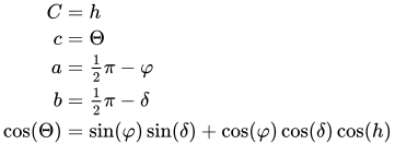
Spherical triangle for application of the spherical law of cosines for calculating the solar zenith angle Θ of an observer at latitude φ and longitude λ, using the hour angle h and solar declination δ (where δ is latitude of subsolar point, and h is relative longitude of subsolar point)

The average annual solar radiation arriving at the top of the Earth's atmosphere is about 1361 W/m². This represents the power per unit area of solar irradiance across the spherical surface surrounding the Sun with a radius equal to the distance to the Earth (1 AU). This means that the approximately circular disc of the Earth, as viewed from the Sun, receives a roughly stable 1361 W/m² at all times. The area of this circular disc is πr², in which r is the radius of the Earth. Because the Earth is approximately spherical, it has total area ${\displaystyle 4\pi r^2}$, meaning that the solar radiation arriving at the top of the atmosphere, averaged over the entire surface of the Earth, is simply divided by four to get 340 W/m². In other words, averaged over the year and the day, the Earth's atmosphere receives 340 W/m² from the Sun. This figure is important in radiative forcing.

Derivation

The distribution of solar radiation at the top of the atmosphere is determined by Earth's sphericity and orbital parameters. This applies to any unidirectional beam incident to a rotating sphere. Insolation is essential for numerical weather prediction and understanding seasons and climatic change. Application to ice ages is known as Milankovitch cycles.

Distribution is based on a fundamental identity from spherical trigonometry, the spherical law of cosines: $${\displaystyle \cos (c)=\cos (a)\cos (b)+\sin (a)\sin (b)\cos (C)}$$ where a, b and c are arc lengths, in radians, of the sides of a spherical triangle. C is the angle in the vertex opposite the side which has arc length c. Applied to the calculation of solar zenith angle Θ, the following applies to the spherical law of cosines: $${\displaystyle \begin{array}{rl}C& =h\\ c& =\mathrm{\Theta }\\ a& =\frac{1}{2}\pi -\phi \\ b& =\frac{1}{2}\pi -\delta \\ \cos (\mathrm{\Theta })& =\sin (\phi )\sin (\delta )+\cos (\phi )\cos (\delta )\cos (h)\end{array}}$$

This equation can be also derived from a more general formula:$${\displaystyle \begin{array}{rl}\cos (\mathrm{\Theta })=\sin (\phi )\sin (\delta )\cos (\beta )& +\sin (\delta )\cos (\phi )\sin (\beta )\cos (\gamma )+\cos (\phi )\cos (\delta )\cos (\beta )\cos (h)\\ & -\cos (\delta )\sin (\phi )\sin (\beta )\cos (\gamma )\cos (h)-\cos (\delta )\sin (\beta )\sin (\gamma )\sin (h)\end{array}}$$ where β is an angle from the horizontal and γ is the solar azimuth angle.

The derivation of the cosine of solar zenith angle, ${\displaystyle \cos (\mathrm{\Theta })}$, based on vector analysis instead of spherical trigonometry is also available in the article about solar azimuth angle.

${\displaystyle {\overline{Q}}^{\text{day}}}$, the theoretical daily-average irradiation at the top of the atmosphere, where θ is the polar angle of the Earth's orbit, and θ = 0 at the March equinox, and θ = 90° at the June solstice; φ is the latitude of the Earth. The calculation assumed conditions appropriate for 2000 A.D.: a solar constant of S₀ = 1367 W m⁻², obliquity of ε = 23.4398°, longitude of perihelion of ϖ = 282.895°, eccentricity e = 0.016704. Contour labels (green) are in units of W m⁻².

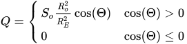
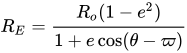
The separation of Earth from the Sun can be denoted R_E and the mean distance can be denoted R₀, approximately 1 astronomical unit (AU). The solar constant is denoted S₀. The solar flux density (insolation) onto a plane tangent to the sphere of the Earth, but above the bulk of the atmosphere (elevation 100 km or greater) is: $${\displaystyle Q=\{\begin{array}{ll}{S}_o\frac{R_o^2}{R_E^2}\cos (\mathrm{\Theta })& \cos (\mathrm{\Theta })>0\\ 0& \cos (\mathrm{\Theta })\le 0\end{array}}$$

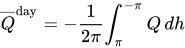
The average of Q over a day is the average of Q over one rotation, or the hour angle progressing from h = π to h = −π: $${\displaystyle {\overline{Q}}^{\text{day}}=-\frac{1}{2\pi }{\int }_{\pi }^{-\pi }Qdh}$$

Let h₀ be the hour angle when Q becomes positive. This could occur at sunrise when ${\displaystyle \mathrm{\Theta }=\frac{1}{2}\pi }$, or for h₀ as a solution of $${\displaystyle \sin (\phi )\sin (\delta )+\cos (\phi )\cos (\delta )\cos (h_o)=0}$$ or $${\displaystyle \cos (h_o)=-\tan (\phi )\tan (\delta )}$$

If tan(φ) tan(δ) > 1, then the sun does not set and the sun is already risen at h = π, so h_o = π. If tan(φ) tan(δ) < −1, the sun does not rise and ${\displaystyle {\overline{Q}}^{\text{day}}=0}$.

${\displaystyle \frac{R_o^2}{R_E^2}}$ is nearly constant over the course of a day, and can be taken outside the integral

$${\displaystyle \begin{array}{rl}{\int }_{\pi }^{-\pi }Qdh& ={\int }_{h_o}^{-h_o}Qdh\\ & =S_o\frac{R_o^2}{R_E^2}{\int }_{h_o}^{-h_o}\cos (\mathrm{\Theta })dh\\ & =S_o\frac{R_o^2}{R_E^2}[h\sin (\phi )\sin (\delta )+\cos (\phi )\cos (\delta )\sin (h){]}_{h=h_o}^{h=-h_o}\\ & =-2S_o\frac{R_o^2}{R_E^2}\left[h_o\sin (\phi )\sin (\delta )+\cos (\phi )\cos (\delta )\sin (h_o)\right]\end{array}}$$

Therefore: $${\displaystyle {\overline{Q}}^{\text{day}}=\frac{S_o}{\pi }\frac{R_o^2}{R_E^2}\left[h_o\sin (\phi )\sin (\delta )+\cos (\phi )\cos (\delta )\sin (h_o)\right]}$$

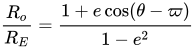
Let θ be the conventional polar angle describing a planetary orbit. Let θ = 0 at the March equinox. The declination δ as a function of orbital position is $${\displaystyle \delta =\epsilon \sin (\theta )}$$ where ε is the obliquity. (Note: The correct formula, valid for any axial tilt, is ${\displaystyle \sin (\delta )=\sin (\epsilon )\sin (\theta )}$.) The conventional longitude of perihelion ϖ is defined relative to the March equinox, so for the elliptical orbit: $${\displaystyle R_E=\frac{R_o(1-e^2)}{1+e\cos (\theta -\varpi )}}$$ or $${\displaystyle \frac{R_o}{R_E}=\frac{1+e\cos (\theta -\varpi )}{1-e^2}}$$

With knowledge of ϖ, ε and e from astrodynamical calculations and S_o from a consensus of observations or theory, ${\displaystyle {\overline{Q}}^{\text{day}}}$can be calculated for any latitude φ and θ. Because of the elliptical orbit, and as a consequence of Kepler's second law, θ does not progress uniformly with time. Nevertheless, θ = 0° is exactly the time of the March equinox, θ = 90° is exactly the time of the June solstice, θ = 180° is exactly the time of the September equinox and θ = 270° is exactly the time of the December solstice.

A simplified equation for irradiance on a given day is:  $${\displaystyle Q\approx S_0\left(1+0.034\cos \left(2\pi \frac{n}{365.25}\right)\right)}$$

where n is a number of a day of the year.

Variation

Total solar irradiance (TSI) changes slowly on decadal and longer timescales. The variation during solar cycle 21 was about 0.1% (peak-to-peak). In contrast to older reconstructions, most recent TSI reconstructions point to an increase of only about 0.05% to 0.1% between the 17th century Maunder Minimum and the present. However, current understanding based on various lines of evidence suggests that the lower values for the secular trend are more probable. In particular, a secular trend greater than 2 Wm⁻² is considered highly unlikely. Ultraviolet irradiance (EUV) varies by approximately 1.5 percent from solar maxima to minima, for 200 to 300 nm wavelengths. However, a proxy study estimated that UV has increased by 3.0% since the Maunder Minimum.

Variations in Earth's orbit, resulting changes in solar energy flux at high latitude, and the observed glacial cycles

Some variations in insolation are not due to solar changes but rather due to the Earth moving between its perihelion and aphelion, or changes in the latitudinal distribution of radiation. These orbital changes or Milankovitch cycles have caused radiance variations of as much as 25% (locally; global average changes are much smaller) over long periods. The most recent significant event was an axial tilt of 24° during boreal summer near the Holocene climatic optimum. Obtaining a time series for a ${\displaystyle {\overline{Q}}^{\mathrm{d}\mathrm{a}\mathrm{y}}}$ for a particular time of year, and particular latitude, is a useful application in the theory of Milankovitch cycles. For example, at the summer solstice, the declination δ is equal to the obliquity ε. The distance from the Sun is $${\displaystyle \frac{R_o}{R_E}=1+e\cos (\theta -\varpi )=1+e\cos \left(\frac{\pi }{2}-\varpi \right)=1+e\sin (\varpi )}$$

For this summer solstice calculation, the role of the elliptical orbit is entirely contained within the important product ${\displaystyle e\sin (\varpi )}$, the precession index, whose variation dominates the variations in insolation at 65° N when eccentricity is large. For the next 100,000 years, with variations in eccentricity being relatively small, variations in obliquity dominate.

Measurement

The space-based TSI record comprises measurements from more than ten radiometers and spans three solar cycles. All modern TSI satellite instruments employ active cavity electrical substitution radiometry. This technique measures the electrical heating needed to maintain an absorptive blackened cavity in thermal equilibrium with the incident sunlight which passes through a precision aperture of calibrated area. The aperture is modulated via a shutter. Accuracy uncertainties of < 0.01% are required to detect long term solar irradiance variations, because expected changes are in the range 0.05–0.15 W/m² per century.

Intertemporal calibration

In orbit, radiometric calibrations drift for reasons including solar degradation of the cavity, electronic degradation of the heater, surface degradation of the precision aperture and varying surface emissions and temperatures that alter thermal backgrounds. These calibrations require compensation to preserve consistent measurements.

For various reasons, the sources do not always agree. The Solar Radiation and Climate Experiment/Total Irradiance Measurement (SORCE/TIM) TSI values are lower than prior measurements by the Earth Radiometer Budget Experiment (ERBE) on the Earth Radiation Budget Satellite (ERBS), VIRGO on the Solar Heliospheric Observatory (SoHO) and the ACRIM instruments on the Solar Maximum Mission (SMM), Upper Atmosphere Research Satellite (UARS) and ACRIMSAT. Pre-launch ground calibrations relied on component rather than system-level measurements since irradiance standards at the time lacked sufficient absolute accuracies.

Measurement stability involves exposing different radiometer cavities to different accumulations of solar radiation to quantify exposure-dependent degradation effects. These effects are then compensated for in the final data. Observation overlaps permits corrections for both absolute offsets and validation of instrumental drifts.

Uncertainties of individual observations exceed irradiance variability (~0.1%). Thus, instrument stability and measurement continuity are relied upon to compute real variations.

Long-term radiometer drifts can potentially be mistaken for irradiance variations which can be misinterpreted as affecting climate. Examples include the issue of the irradiance increase between cycle minima in 1986 and 1996, evident only in the ACRIM composite (and not the model) and the low irradiance levels in the PMOD composite during the 2008 minimum.

Despite the fact that ACRIM I, ACRIM II, ACRIM III, VIRGO and TIM all track degradation with redundant cavities, notable and unexplained differences remain in irradiance and the modeled influences of sunspots and faculae.

Persistent inconsistencies

Disagreement among overlapping observations indicates unresolved drifts that suggest the TSI record is not sufficiently stable to discern solar changes on decadal time scales. Only the ACRIM composite shows irradiance increasing by ~1 W/m² between 1986 and 1996. It is noteworthy that the most accurate TSI reconstructions with empirical and physics-based semi-empirical models using independent inputs consistently disfavor this increase during the ACRIM-gap.

Recommendations to resolve the instrument discrepancies include validating optical measurement accuracy by comparing ground-based instruments to laboratory references, such as those at National Institute of Science and Technology (NIST); NIST validation of aperture area calibrations uses spares from each instrument; and applying diffraction corrections from the view-limiting aperture.

For ACRIM, NIST determined that diffraction from the view-limiting aperture contributes a 0.13% signal not accounted for in the three ACRIM instruments. This correction lowers the reported ACRIM values, bringing ACRIM closer to TIM. In ACRIM and all other instruments but TIM, the aperture is deep inside the instrument, with a larger view-limiting aperture at the front. Depending on edge imperfections this can directly scatter light into the cavity. This design admits into the front part of the instrument two to three times the amount of light intended to be measured; if not completely absorbed or scattered, this additional light produces erroneously high signals. In contrast, TIM's design places the precision aperture at the front so that only desired light enters.

Variations from other sources likely include an annual systematics in the ACRIM III data that is nearly in phase with the Sun-Earth distance and 90-day spikes in the VIRGO data coincident with SoHO spacecraft maneuvers that were most apparent during the 2008 solar minimum.

TSI Radiometer Facility

TIM's high absolute accuracy creates new opportunities for measuring climate variables. TSI Radiometer Facility (TRF) is a cryogenic radiometer that operates in a vacuum with controlled light sources. L-1 Standards and Technology (LASP) designed and built the system, completed in 2008. It was calibrated for optical power against the NIST Primary Optical Watt Radiometer, a cryogenic radiometer that maintains the NIST radiant power scale to an uncertainty of 0.02% (1σ). As of 2011 TRF was the only facility that approached the desired <0.01% uncertainty for pre-launch validation of solar radiometers measuring irradiance (rather than merely optical power) at solar power levels and under vacuum conditions.

TRF encloses both the reference radiometer and the instrument under test in a common vacuum system that contains a stationary, spatially uniform illuminating beam. A precision aperture with an area calibrated to 0.0031% (1σ) determines the beam's measured portion. The test instrument's precision aperture is positioned in the same location, without optically altering the beam, for direct comparison to the reference. Variable beam power provides linearity diagnostics, and variable beam diameter diagnoses scattering from different instrument components.

The Glory/TIM and PICARD/PREMOS flight instrument absolute scales are now traceable to the TRF in both optical power and irradiance. The resulting high accuracy reduces the consequences of any future gap in the solar irradiance record.

Difference relative to TRF

Instrument	Irradiance, view-limiting aperture overfilled	Irradiance, precision aperture overfilled	Difference attributable to scatter error	Measured optical power error	Residual irradiance agreement	Uncertainty
SORCE/TIM ground	—N/a	−0.037%	—N/a	−0.037%	0.000%	0.032%
Glory/TIM flight	—N/a	−0.012%	—N/a	−0.029%	0.017%	0.020%
PREMOS-1 ground	−0.005%	−0.104%	0.098%	−0.049%	−0.104%	~0.038%
PREMOS-3 flight	0.642%	0.605%	0.037%	0.631%	−0.026%	~0.027%
VIRGO-2 ground	0.897%	0.743%	0.154%	0.730%	0.013%	~0.025%

2011 reassessment

The most probable value of TSI representative of solar minimum is 1360.9±0.5 W/m², lower than the earlier accepted value of 1365.4±1.3 W/m², established in the 1990s. The new value came from SORCE/TIM and radiometric laboratory tests. Scattered light is a primary cause of the higher irradiance values measured by earlier satellites in which the precision aperture is located behind a larger, view-limiting aperture. The TIM uses a view-limiting aperture that is smaller than the precision aperture that precludes this spurious signal. The new estimate is from better measurement rather than a change in solar output.

A regression model-based split of the relative proportion of sunspot and facular influences from SORCE/TIM data accounts for 92% of observed variance and tracks the observed trends to within TIM's stability band. This agreement provides further evidence that TSI variations are primarily due to solar surface magnetic activity.

Instrument inaccuracies add a significant uncertainty in determining Earth's energy balance. The energy imbalance has been variously measured (during a deep solar minimum of 2005–2010) to be +0.58±0.15 W/m², +0.60±0.17 W/m² and +0.85 W/m². Estimates from space-based measurements range +3–7 W/m². SORCE/TIM's lower TSI value reduces this discrepancy by 1 W/m². This difference between the new lower TIM value and earlier TSI measurements corresponds to a climate forcing of −0.8 W/m², which is comparable to the energy imbalance.

On Earth's surface

A pyranometer, used to measure global irradiance

A pyrheliometer, mounted on a solar tracker, is used to measure Direct Normal Irradiance (or beam irradiance).

Average annual solar radiation arriving at the top of the Earth's atmosphere is roughly 1361 W/m². The Sun's rays are attenuated as they pass through the atmosphere, leaving maximum normal surface irradiance at approximately 1000 W/m² at sea level on a clear day. When 1361 W/m² is arriving above the atmosphere (when the Sun is at the zenith in a cloudless sky), direct sun is about 1050 W/m², and global radiation on a horizontal surface at ground level is about 1120 W/m². The latter figure includes radiation scattered or reemitted by the atmosphere and surroundings. The actual figure varies with the Sun's angle and atmospheric circumstances. Ignoring clouds, the daily average insolation for the Earth is approximately 6 kWh/m² = 21.6 MJ/m².

The output of, for example, a photovoltaic panel, partly depends on the angle of the sun relative to the panel. One Sun is a unit of power flux, not a standard value for actual insolation. Sometimes this unit is referred to as a Sol, not to be confused with a sol, meaning one solar day.

Absorption and reflection

Solar irradiance spectrum above atmosphere and at surface

Part of the radiation reaching an object is absorbed and the remainder reflected. Usually, the absorbed radiation is converted to thermal energy, increasing the object's temperature. Humanmade or natural systems, however, can convert part of the absorbed radiation into another form such as electricity or chemical bonds, as in the case of photovoltaic cells or plants. The proportion of reflected radiation is the object's reflectivity or albedo.

Projection effect

Projection effect: One sunbeam one mile wide shines on the ground at a 90° angle, and another at a 30° angle. The oblique sunbeam distributes its light energy over twice as much area.

Insolation onto a surface is largest when the surface directly faces (is normal to) the sun. As the angle between the surface and the Sun moves from normal, the insolation is reduced in proportion to the angle's cosine; see effect of Sun angle on climate.

In the figure, the angle shown is between the ground and the sunbeam rather than between the vertical direction and the sunbeam; hence the sine rather than the cosine is appropriate. A sunbeam one mile wide arrives from directly overhead, and another at a 30° angle to the horizontal. The sine of a 30° angle is 1/2, whereas the sine of a 90° angle is 1. Therefore, the angled sunbeam spreads the light over twice the area. Consequently, half as much light falls on each square mile.

This projection effect is the main reason why Earth's polar regions are much colder than equatorial regions. On an annual average, the poles receive less insolation than does the equator, because the poles are always angled more away from the Sun than the tropics, and moreover receive no insolation at all for the six months of their respective winters.

Absorption effect

At a lower angle, the light must also travel through more atmosphere. This attenuates it (by absorption and scattering) further reducing insolation at the surface.

Attenuation is governed by the Beer-Lambert Law, namely that the transmittance or fraction of insolation reaching the surface decreases exponentially in the optical depth or absorbance (the two notions differing only by a constant factor of ln(10) = 2.303) of the path of insolation through the atmosphere. For any given short length of the path, the optical depth is proportional to the number of absorbers and scatterers along that length, typically increasing with decreasing altitude. The optical depth of the whole path is then the integral (sum) of those optical depths along the path.

When the density of absorbers is layered, that is, depends much more on vertical than horizontal position in the atmosphere, to a good approximation the optical depth is inversely proportional to the projection effect, that is, to the cosine of the zenith angle. Since transmittance decreases exponentially with increasing optical depth, as the sun approaches the horizon there comes a point when absorption dominates projection for the rest of the day. With a relatively high level of absorbers this can be a considerable portion of the late afternoon, and likewise of the early morning. Conversely, in the (hypothetical) total absence of absorption, the optical depth remains zero at all altitudes of the sun, that is, transmittance remains 1, and so only the projection effect applies.

Solar potential maps

Assessment and mapping of solar potential at the global, regional and country levels have been the subject of significant academic and commercial interest. One of the earliest attempts to carry out comprehensive mapping of solar potential for individual countries was the Solar & Wind Resource Assessment (SWERA) project, funded by the United Nations Environment Program and carried out by the US National Renewable Energy Laboratory (NREL). The National Aeronautics and Space Administration (NASA) provides data for global solar potential maps through the CERES experiment and the POWER project. Global mapping by many other similar institutes are available on the Global Atlas for Renewable Energy provided by the International Renewable Energy Agency. 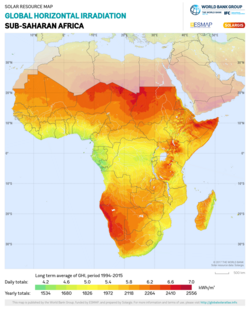A number of commercial firms now exist to provide solar resource data to solar power developers, including 3E, Clean Power Research, SoDa Solar Radiation Data, Solargis, Vaisala (previously 3Tier), and Vortex, and these firms have often provided solar potential maps for free. The Global Solar Atlas was launched by the World Bank in January 2017, using data provided by Solargis, to provide a single source for high-quality solar data, maps, and GIS layers covering all countries.

• Maps of GHI potential by region and country (Note: colors are not consistent across maps)
• 
  Sub-Saharan Africa
   
• 
  Latin America and Caribbean
   
• 
  China
   
• 
  India
   
• 
  Mexico
• 
  South Africa

Solar radiation maps are built using databases derived from satellite imagery, as for example using visible images from Meteosat Prime satellite. A method is applied to the images to determine solar radiation. One well validated satellite-to-irradiance model is the SUNY model. The accuracy of this model is well evaluated. In general, solar irradiance maps are accurate, especially for Global Horizontal Irradiance.

Applications

Solar power

Sunlight carries radiant energy in the wavelengths of visible light. Radiant energy may be developed for solar power generation.

Solar irradiation figures are used to plan the deployment of solar power systems. In many countries, the figures can be obtained from an insolation map or from insolation tables that reflect data over the prior 30–50 years. Different solar power technologies are able to use different components of the total irradiation. While solar photovoltaics panels are able to convert to electricity both direct irradiation and diffuse irradiation, concentrated solar power is only able to operate efficiently with direct irradiation, thus making these systems suitable only in locations with relatively low cloud cover.

Because solar collectors panels are almost always mounted at an angle towards the Sun, insolation figures must be adjusted to find the amount of sunlight falling on the panel. This will prevent estimates that are inaccurately low for winter and inaccurately high for summer. This also means that the amount of sunlight falling on a solar panel at high latitude is not as low compared to one at the equator as would appear from just considering insolation on a horizontal surface. Horizontal insolation values range from 800 to 950 kWh/(kWp·y) in Norway to up to 2,900 kWh/(kWp·y) in Australia. But a properly tilted panel at 50° latitude receives 1860 kWh/m²/y, compared to 2370 at the equator. In fact, under clear skies a solar panel placed horizontally at the north or south pole at midsummer receives more sunlight over 24 hours (cosine of angle of incidence equal to sin(23.5°) or about 0.40) than a horizontal panel at the equator at the equinox (average cosine equal to 1/π or about 0.32).

Photovoltaic panels are rated under standard conditions to determine the Wp (peak watts) rating, which can then be used with insolation, adjusted by factors such as tilt, tracking and shading, to determine the expected output.

Buildings

Insolation variation by month; 1984–1993 averages for January (top) and April (bottom)

In construction, insolation is an important consideration when designing a building for a particular site.

The projection effect can be used to design buildings that are cool in summer and warm in winter, by providing vertical windows on the equator-facing side of the building (the south face in the Northern Hemisphere, or the north face in the Southern Hemisphere): this maximizes insolation in the winter months when the Sun is low in the sky and minimizes it in the summer when the Sun is high. (The Sun's north–south path through the sky spans 47° through the year).

Civil engineering

In civil engineering and hydrology, numerical models of snowmelt runoff use observations of insolation. This permits estimation of the rate at which water is released from a melting snowpack. Field measurement is accomplished using a pyranometer.

Climate research

Irradiance plays a part in climate modeling and weather forecasting. A non-zero average global net radiation at the top of the atmosphere is indicative of Earth's thermal disequilibrium as imposed by climate forcing.

The impact of the lower 2014 TSI value on climate models is unknown. A few tenths of a percent change in the absolute TSI level is typically considered to be of minimal consequence for climate simulations. The new measurements require climate model parameter adjustments.

Experiments with GISS Model 3 investigated the sensitivity of model performance to the TSI absolute value during the present and pre-industrial epochs, and describe, for example, how the irradiance reduction is partitioned between the atmosphere and surface and the effects on outgoing radiation.

Assessing the impact of long-term irradiance changes on climate requires greater instrument stability combined with reliable global surface temperature observations to quantify climate response processes to radiative forcing on decadal time scales. The observed 0.1% irradiance increase imparts 0.22 W/m² climate forcing, which suggests a transient climate response of 0.6 °C per W/m². This response is larger by a factor of 2 or more than in the IPCC-assessed 2008 models, possibly appearing in the models' heat uptake by the ocean.

Global cooling

Measuring a surface's capacity to reflect solar irradiance is essential to passive daytime radiative cooling, which has been proposed as a method of reversing local and global temperature increases associated with global warming. In order to measure the cooling power of a passive radiative cooling surface, both the absorbed powers of atmospheric and solar radiations must be quantified. On a clear day, solar irradiance can reach 1000 W/m² with a diffuse component between 50 and 100 W/m². On average the cooling power of a passive daytime radiative cooling surface has been estimated at ~100-150 W/m².

Space

Insolation is the primary variable affecting equilibrium temperature in spacecraft design and planetology.

Solar activity and irradiance measurement is a concern for space travel. For example, the American space agency, NASA, launched its Solar Radiation and Climate Experiment (SORCE) satellite with Solar Irradiance Monitors.

Energy flow (ecology)

From Wikipedia, the free encyclopedia

https://en.wikipedia.org/wiki/Energy_flow_(ecology)

A food pyramid and a corresponding food web, demonstrating some of the simpler patterns in a food web

A graphic representation of energy transfer between trophic layers in an ecosystem

Energy flow is the flow of energy through living things within an ecosystem. All living organisms can be organized into producers and consumers, and those producers and consumers can further be organized into a food chain. Each of the levels within the food chain is a trophic level. In order to more efficiently show the quantity of organisms at each trophic level, these food chains are then organized into trophic pyramids. The arrows in the food chain show that the energy flow is unidirectional, with the head of an arrow indicating the direction of energy flow; energy is lost as heat at each step along the way.

The unidirectional flow of energy and the successive loss of energy as it travels up the food web are patterns in energy flow that are governed by thermodynamics, which is the theory of energy exchange between systems. Trophic dynamics relates to thermodynamics because it deals with the transfer and transformation of energy (originating externally from the sun via solar radiation) to and among organisms.

Energetics and the carbon cycle

The carbon cycle of a terrestrial ecosystem. Beginning with photosynthesis, water (blue) and carbon dioxide (white) from the air are taken in with solar energy (yellow), and are converted into plant energy (green). 100×10¹⁵ grams of carbon/year fixed by photosynthetic organisms, which is equivalent to 4×10¹⁸ kJ/yr = 4×10²¹ J/yr of free energy. Cellular respiration is the reverse reaction, wherein energy of plants is taken in and carbon dioxide and water are given off. The carbon dioxide and water produced can be recycled back into plants.

The first step in energetics is photosynthesis, where in water and carbon dioxide from the air are taken in with energy from the sun, and are converted into oxygen and glucose. Cellular respiration is the reverse reaction, wherein oxygen and sugar are taken in and release energy as they are converted back into carbon dioxide and water. The carbon dioxide and water produced by respiration can be recycled back into plants.

Energy loss can be measured either by efficiency (how much energy makes it to the next level), or by biomass (how much living material exists at those levels at one point in time, measured by standing crop). Of all the net primary productivity at the producer trophic level, in general only 10% goes to the next level, the primary consumers, then only 10% of that 10% goes on to the next trophic level, and so on up the food pyramid. Ecological efficiency may be anywhere from 5% to 20% depending on how efficient or inefficient that ecosystem is. This decrease in efficiency occurs because organisms need to perform cellular respiration to survive, and energy is lost as heat when cellular respiration is performed. That is also why there are fewer tertiary consumers than there are producers.

Primary production

Main article: Primary production

Fate of mangrove primary production

A producer is any organism that performs photosynthesis. Producers are important because they convert energy from the sun into a storable and usable chemical form of energy, glucose, as well as oxygen. The producers themselves can use the energy stored in glucose to perform cellular respiration. Or, if the producer is consumed by herbivores in the next trophic level, some of the energy is passed on up the pyramid. The glucose stored within producers serves as food for consumers, and so it is only through producers that consumers are able to access the sun's energy. Some examples of primary producers are algae, mosses, and other plants such as grasses, trees, and shrubs.

Chemosynthetic bacteria perform a process similar to photosynthesis, but instead of energy from the sun they use energy stored in chemicals like hydrogen sulfide. This process, referred to as chemosynthesis, usually occurs deep in the ocean at hydrothermal vents that produce heat and chemicals such as hydrogen, hydrogen sulfide and methane. Chemosynthetic bacteria can use the energy in the bonds of the hydrogen sulfide and oxygen to convert carbon dioxide to glucose, releasing water and sulfur in the process. Organisms that consume the chemosynthetic bacteria can take in the glucose and use oxygen to perform cellular respiration, similar to herbivores consuming producers.

One of the factors that controls primary production is the amount of energy that enters the producer(s), which can be measured using productivity. Only one percent of solar energy enters the producer, the rest bounces off or moves through. Gross primary productivity is the amount of energy the producer actually gets. Generally, 60% of the energy that enters the producer goes to the producer's own respiration. The net primary productivity is the amount that the plant retains after the amount that it used for cellular respiration is subtracted. Another factor controlling primary production is organic/inorganic nutrient levels in the water or soil that the producer is living in. An example of the nutrients that can impact the efficiency of primary plant production are nitrogen (N) and phosphorus (P).

Venus Flytrap

Carnivorous plants

When it comes to dealing with environments that have low nutrient availability, some plants have developed unique ways to adapt to be able to perform photosynthesis. In order to do so, these plants have evolved to be able to obtain important nutrients such as nitrogen from other organisms, just as heterotrophs would giving them the unique title of carnivorous plants. With methods such as the pitfall trap (pitcher plant), the flypaper trap (Drosera capensis), or the snap trap (venus flytrap) these plants have learned to lure insects in and digest them.

Pitcher plants lure insects in using a variety of attractive cues such as scent and color. Once an insect or small organism falls into the bulb shaped body of the plant, a variety of enzymes are secreted beginning the digestion process of the organism and preventing it from escaping. Flypaper trap plants, the most common of carnivorous plants, secret a special liquid that allow an insect to land on its leaves but then prevents the insect from escaping. The snap trap plant, use similar methods to the pitcher plant in order to attract various insects. However, these carnivorous plants are able to detect when an insect is touching its leaves thus triggering the "mouth" of the plant to close and encase the insect. In developing this method of nutrient acquisition, carnivorous plants are able to survive in almost any environment around the world, excluding Antarctica and the Arctic Circle.

Secondary production

Secondary production is the use of energy stored in plants converted by consumers to their own biomass. Different ecosystems have different levels of consumers, all end with one top consumer. Most energy is stored in organic matter of plants, and as the consumers eat these plants they take up this energy. This energy in the herbivores and omnivores is then consumed by carnivores. There is also a large amount of energy that is in primary production and ends up being waste or litter, referred to as detritus. The detrital food chain includes a large amount of microbes, macroinvertebrates, meiofauna, fungi, and bacteria. These organisms are consumed by omnivores and carnivores and account for a large amount of secondary production. Secondary consumers can vary widely in how efficient they are in consuming. The efficiency of energy being passed on to consumers is estimated to be around 10%. Energy flow through consumers differs in aquatic and terrestrial environments.

In aquatic environments

Heterotrophs contribute to secondary production and it is dependent on primary productivity and the net primary products. Secondary production is the energy that herbivores and decomposers use and thus depends on primary productivity. Primarily herbivores and decomposers consume all the carbon from two main organic sources in aquatic ecosystems, autochthonous and allochthonous. Autochthonous carbon comes from within the ecosystem and includes aquatic plants, algae and phytoplankton. Allochthonous carbon from outside the ecosystem is mostly dead organic matter from the terrestrial ecosystem entering the water. In stream ecosystems, approximately 66% of annual energy input can be washed downstream. The remaining amount is consumed and lost as heat.

In terrestrial environments

Secondary production is often described in terms of trophic levels, and while this can be useful in explaining relationships it overemphasizes the rarer interactions. Consumers often feed at multiple trophic levels. Energy transferred above the third trophic level is relatively unimportant. The assimilation efficiency can be expressed by the amount of food the consumer has eaten, how much the consumer assimilates and what is expelled as feces or urine. While a portion of the energy is used for respiration, another portion of the energy goes towards biomass in the consumer. There are two major food chains: The primary food chain is the energy coming from autotrophs and passed on to the consumers; and the second major food chain is when carnivores eat the herbivores or decomposers that consume the autotrophic energy. Consumers are broken down into primary consumers, secondary consumers and tertiary consumers. Carnivores have a much higher assimilation of energy, about 80% and herbivores have a much lower efficiency of approximately 20 to 50%. Energy in a system can be affected by animal emigration/immigration. The movements of organisms are significant in terrestrial ecosystems. Energetic consumption by herbivores in terrestrial ecosystems has a low range of ~3-7%. The flow of energy is similar in many terrestrial environments. The fluctuation in the amount of net primary product consumed by herbivores is generally low. This is in large contrast to aquatic environments of lakes and ponds where grazers have a much higher consumption of around ~33%. Ectotherms and endotherms have very different assimilation efficiencies.

Detritivores

Detritivores consume organic material that is decomposing and are in turn consumed by carnivores. Predator productivity is correlated with prey productivity. This confirms that the primary productivity in ecosystems affects all productivity following.

Detritus is a large portion of organic material in ecosystems. Organic material in temperate forests is mostly made up of dead plants, approximately 62%.

In an aquatic ecosystem, leaf matter that falls into streams gets wet and begins to leech organic material. This happens rather quickly and will attract microbes and invertebrates. The leaves can be broken down into large pieces called coarse particulate organic matter (CPOM). The CPOM is rapidly colonized by microbes. Meiofauna is extremely important to secondary production in stream ecosystems. Microbes breaking down and colonizing this leaf matter are very important to the detritovores. The detritovores make the leaf matter more edible by releasing compounds from the tissues; it ultimately helps soften them. As leaves decay nitrogen will decrease since cellulose and lignin in the leaves is difficult to break down. Thus the colonizing microbes bring in nitrogen in order to aid in the decomposition. Leaf breakdown can depend on initial nitrogen content, season, and species of trees. The species of trees can have variation when their leaves fall. Thus the breakdown of leaves is happening at different times, which is called a mosaic of microbial populations.

Species effect and diversity in an ecosystem can be analyzed through their performance and efficiency. In addition, secondary production in streams can be influenced heavily by detritus that falls into the streams; production of benthic fauna biomass and abundance decreased an additional 47–50% during a study of litter removal and exclusion.

Energy flow across ecosystems

Research has demonstrated that primary producers fix carbon at similar rates across ecosystems. Once carbon has been introduced into a system as a viable source of energy, the mechanisms that govern the flow of energy to higher trophic levels vary across ecosystems. Among aquatic and terrestrial ecosystems, patterns have been identified that can account for this variation and have been divided into two main pathways of control: top-down and bottom-up. The acting mechanisms within each pathway ultimately regulate community and trophic level structure within an ecosystem to varying degrees. Bottom-up controls involve mechanisms that are based on resource quality and availability, which control primary productivity and the subsequent flow of energy and biomass to higher trophic levels. Top-down controls involve mechanisms that are based on consumption by consumers. These mechanisms control the rate of energy transfer from one trophic level to another as herbivores or predators feed on lower trophic levels.

Aquatic vs terrestrial ecosystems

Much variation in the flow of energy is found within each type of ecosystem, creating a challenge in identifying variation between ecosystem types. In a general sense, the flow of energy is a function of primary productivity with temperature, water availability, and light availability. For example, among aquatic ecosystems, higher rates of production are usually found in large rivers and shallow lakes than in deep lakes and clear headwater streams. Among terrestrial ecosystems, marshes, swamps, and tropical rainforests have the highest primary production rates, whereas tundra and alpine ecosystems have the lowest. The relationships between primary production and environmental conditions have helped account for variation within ecosystem types, allowing ecologists to demonstrate that energy flows more efficiently through aquatic ecosystems than terrestrial ecosystems due to the various bottom-up and top-down controls in play.

Bottom-up

The strength of bottom-up controls on energy flow are determined by the nutritional quality, size, and growth rates of primary producers in an ecosystem. Photosynthetic material is typically rich in nitrogen (N) and phosphorus (P) and supplements the high herbivore demand for N and P across all ecosystems. Aquatic primary production is dominated by small, single-celled phytoplankton that are mostly composed of photosynthetic material, providing an efficient source of these nutrients for herbivores. In contrast, multi-cellular terrestrial plants contain many large supporting cellulose structures of high carbon but low nutrient value. Because of this structural difference, aquatic primary producers have less biomass per photosynthetic tissue stored within the aquatic ecosystem than in the forests and grasslands of terrestrial ecosystems. This low biomass relative to photosynthetic material in aquatic ecosystems allows for a more efficient turnover rate compared to terrestrial ecosystems. As phytoplankton are consumed by herbivores, their enhanced growth and reproduction rates sufficiently replace lost biomass and, in conjunction with their nutrient dense quality, support greater secondary production.

Additional factors impacting primary production includes inputs of N and P, which occurs at a greater magnitude in aquatic ecosystems. These nutrients are important in stimulating plant growth and, when passed to higher trophic levels, stimulate consumer biomass and growth rate. If either of these nutrients are in short supply, they can limit overall primary production. Within lakes, P tends to be the greater limiting nutrient while both N and P limit primary production in rivers. Due to these limiting effects, nutrient inputs can potentially alleviate the limitations on net primary production of an aquatic ecosystem. Allochthonous material washed into an aquatic ecosystem introduces N and P as well as energy in the form of carbon molecules that are readily taken up by primary producers. Greater inputs and increased nutrient concentrations support greater net primary production rates, which in turn supports greater secondary production.

Top-down

Top-down mechanisms exert greater control on aquatic primary producers due to the roll of consumers within an aquatic food web. Among consumers, herbivores can mediate the impacts of trophic cascades by bridging the flow of energy from primary producers to predators in higher trophic levels. Across ecosystems, there is a consistent association between herbivore growth and producer nutritional quality. However, in aquatic ecosystems, primary producers are consumed by herbivores at a rate four times greater than in terrestrial ecosystems. Although this topic is highly debated, researchers have attributed the distinction in herbivore control to several theories, including producer to consumer size ratios and herbivore selectivity.

A freshwater food web demonstrating the size differences between each trophic level. Primary producers tend to be small algal cells. Herbivores tend to be small macro-invertebrates. Predators tend to be larger fish.

Modeling of top-down controls on primary producers suggests that the greatest control on the flow of energy occurs when the size ratio of consumer to primary producer is the highest. The size distribution of organisms found within a single trophic level in aquatic systems is much narrower than that of terrestrial systems. On land, the consumer size ranges from smaller than the plant it consumes, such as an insect, to significantly larger, such as an ungulate, while in aquatic systems, consumer body size within a trophic level varies much less and is strongly correlated with trophic position. As a result, the size difference between producers and consumers is consistently larger in aquatic environments than on land, resulting in stronger herbivore control over aquatic primary producers.

Herbivores can potentially control the fate of organic matter as it is cycled through the food web. Herbivores tend to select nutritious plants while avoiding plants with structural defense mechanisms. Like support structures, defense structures are composed of nutrient poor, high carbon cellulose. Access to nutritious food sources enhances herbivore metabolism and energy demands, leading to greater removal of primary producers. In aquatic ecosystems, phytoplankton are highly nutritious and generally lack defense mechanisms. This results in greater top-down control because consumed plant matter is quickly released back into the system as labile organic waste. In terrestrial ecosystems, primary producers are less nutritionally dense and are more likely to contain defense structures. Because herbivores prefer nutritionally dense plants and avoid plants or plant parts with defense structures, a greater amount of plant matter is left unconsumed within the ecosystem. Herbivore avoidance of low-quality plant matter may be why terrestrial systems exhibit weaker top-down control on the flow of energy.