Electric field

From Wikipedia, the free encyclopedia
https://en.wikipedia.org/wiki/Electric_field

An electric field (sometimes called E-field) is a physical field that surrounds electrically charged particles such as electrons. In classical electromagnetism, the electric field of a single charge (or group of charges) describes their capacity to exert attractive or repulsive forces on another charged object. Charged particles exert attractive forces on each other when the sign of their charges are opposite, one being positive while the other is negative, and repel each other when the signs of the charges are the same. Because these forces are exerted mutually, two charges must be present for the forces to take place. These forces are described by Coulomb's law, which says that the greater the magnitude of the charges, the greater the force, and the greater the distance between them, the weaker the force. Informally, the greater the charge of an object, the stronger its electric field. Similarly, an electric field is stronger nearer charged objects and weaker further away. Electric fields originate from electric charges and time-varying electric currents. Electric fields and magnetic fields are both manifestations of the electromagnetic field. Electromagnetism is one of the four fundamental interactions of nature.

Electric fields are important in many areas of physics, and are exploited in electrical technology. For example, in atomic physics and chemistry, the interaction in the electric field between the atomic nucleus and electrons is the force that holds these particles together in atoms. Similarly, the interaction in the electric field between atoms is the force responsible for chemical bonding that result in molecules.

The electric field is defined as a vector field that associates to each point in space the force per unit of charge exerted on an infinitesimal positive test charge at rest at that point. The SI unit for the electric field is the volt per meter (V/m), which is equal to the newton per coulomb (N/C).

Description

Electric field of a positive point electric charge suspended over an infinite sheet of conducting material. The field is depicted by electric field lines, lines which follow the direction of the electric field in space. The induced charge distribution in the sheet is not shown.

The electric field is defined at each point in space as the force that would be experienced by an infinitesimally small stationary positive test charge at that point divided by the charge. The electric field is defined in terms of force, and force is a vector (i.e. having both magnitude and direction), so it follows that an electric field may be described by a vector field. The electric field acts between two charges similarly to the way that the gravitational field acts between two masses, as they both obey an inverse-square law with distance. This is the basis for Coulomb's law, which states that, for stationary charges, the electric field varies with the source charge and varies inversely with the square of the distance from the source. This means that if the source charge were doubled, the electric field would double, and if you move twice as far away from the source, the field at that point would be only one-quarter its original strength.

The electric field can be visualized with a set of lines whose direction at each point is the same as those of the field, a concept introduced by Michael Faraday, whose term 'lines of force' is still sometimes used. This illustration has the useful property that, when drawn so that each line represents the same amount of flux, the strength of the field is proportional to the density of the lines. Field lines due to stationary charges have several important properties, including that they always originate from positive charges and terminate at negative charges, they enter all good conductors at right angles, and they never cross or close in on themselves. The field lines are a representative concept; the field actually permeates all the intervening space between the lines. More or fewer lines may be drawn depending on the precision to which it is desired to represent the field. The study of electric fields created by stationary charges is called electrostatics.

Faraday's law describes the relationship between a time-varying magnetic field and the electric field. One way of stating Faraday's law is that the curl of the electric field is equal to the negative time derivative of the magnetic field. In the absence of time-varying magnetic field, the electric field is therefore called conservative (i.e. curl-free). This implies there are two kinds of electric fields: electrostatic fields and fields arising from time-varying magnetic fields. While the curl-free nature of the static electric field allows for a simpler treatment using electrostatics, time-varying magnetic fields are generally treated as a component of a unified electromagnetic field. The study of magnetic and electric fields that change over time is called electrodynamics.

Mathematical formulation

Main article: Mathematical descriptions of the electromagnetic field

Electric fields are caused by electric charges, described by Gauss's law, and time varying magnetic fields, described by Faraday's law of induction. Together, these laws are enough to define the behavior of the electric field. However, since the magnetic field is described as a function of electric field, the equations of both fields are coupled and together form Maxwell's equations that describe both fields as a function of charges and currents.

Evidence of an electric field: styrofoam peanuts clinging to a cat's fur due to static electricity. The triboelectric effect causes an electrostatic charge to build up on the fur due to the cat's motions. The electric field of the charge causes polarization of the molecules of the styrofoam due to electrostatic induction, resulting in a slight attraction of the light plastic pieces to the charged fur. This effect is also the cause of static cling in clothes.

Electrostatics

Main article: Coulomb's law

In the special case of a steady state (stationary charges and currents), the Maxwell-Faraday inductive effect disappears. The resulting two equations (Gauss's law ${\displaystyle \mathrm{\nabla }\cdot \mathbf{E}=\frac{\rho }{{\epsilon }_0}}$ and Faraday's law with no induction term ${\displaystyle \mathrm{\nabla }\times \mathbf{E}=0}$), taken together, are equivalent to Coulomb's law, which states that a particle with electric charge ${\displaystyle q_1}$ at position ${\displaystyle {\mathbf{r}}_1}$ exerts a force on a particle with charge ${\displaystyle q_0}$ at position ${\displaystyle {\mathbf{r}}_0}$ of: $${\displaystyle {\mathbf{F}}_{01}=\frac{q_1{q}_0}{4\pi {\epsilon }_0}\frac{{\hat{\mathbf{r}}}_{01}}{{|{\mathbf{r}}_{01}|}^2}=\frac{q_1{q}_0}{4\pi {\epsilon }_0}\frac{{\mathbf{r}}_{01}}{{|{\mathbf{r}}_{01}|}^3}}$$ where

• ${\displaystyle {\mathbf{F}}_{01}}$ is the force on charged particle ${\displaystyle q_0}$ caused by charged particle ${\displaystyle q_1}$.
• ε₀ is the permittivity of free space.
• ${\displaystyle {\hat{\mathbf{r}}}_{01}}$ is a unit vector directed from ${\displaystyle {\mathbf{r}}_1}$ to ${\displaystyle {\mathbf{r}}_0}$.
• ${\displaystyle {\mathbf{r}}_{01}}$ is the displacement vector from ${\displaystyle {\mathbf{r}}_1}$ to ${\displaystyle {\mathbf{r}}_0}$.

Note that ${\displaystyle {\epsilon }_0}$ must be replaced with ${\displaystyle \epsilon }$, permittivity, when charges are in non-empty media. When the charges ${\displaystyle q_0}$ and ${\displaystyle q_1}$ have the same sign this force is positive, directed away from the other charge, indicating the particles repel each other. When the charges have unlike signs the force is negative, indicating the particles attract. To make it easy to calculate the Coulomb force on any charge at position ${\displaystyle {\mathbf{r}}_0}$ this expression can be divided by ${\displaystyle q_0}$ leaving an expression that only depends on the other charge (the source charge) $${\displaystyle {\mathbf{E}}_1({\mathbf{r}}_0)=\frac{{\mathbf{F}}_{01}}{q_0}=\frac{q_1}{4\pi {\epsilon }_0}\frac{{\hat{\mathbf{r}}}_{01}}{{|{\mathbf{r}}_{01}|}^2}=\frac{q_1}{4\pi {\epsilon }_0}\frac{{\mathbf{r}}_{01}}{{|{\mathbf{r}}_{01}|}^3}}$$ where ${\displaystyle {\mathbf{E}}_1({\mathbf{r}}_0)}$ is the component of the electric field at ${\displaystyle q_0}$ due to ${\displaystyle q_1}$.

This is the electric field at point ${\displaystyle {\mathbf{r}}_0}$ due to the point charge ${\displaystyle q_1}$; it is a vector-valued function equal to the Coulomb force per unit charge that a positive point charge would experience at the position ${\displaystyle {\mathbf{r}}_0}$. Since this formula gives the electric field magnitude and direction at any point ${\displaystyle {\mathbf{r}}_0}$ in space (except at the location of the charge itself, ${\displaystyle {\mathbf{r}}_1}$, where it becomes infinite) it defines a vector field. From the above formula it can be seen that the electric field due to a point charge is everywhere directed away from the charge if it is positive, and toward the charge if it is negative, and its magnitude decreases with the inverse square of the distance from the charge.

The Coulomb force on a charge of magnitude ${\displaystyle q}$ at any point in space is equal to the product of the charge and the electric field at that point $${\displaystyle \mathbf{F}=q\mathbf{E}.}$$ The SI unit of the electric field is the newton per coulomb (N/C), or volt per meter (V/m); in terms of the SI base units it is kg⋅m⋅s⁻³⋅A⁻¹.

Superposition principle

Due to the linearity of Maxwell's equations, electric fields satisfy the superposition principle, which states that the total electric field, at a point, due to a collection of charges is equal to the vector sum of the electric fields at that point due to the individual charges. This principle is useful in calculating the field created by multiple point charges. If charges ${\displaystyle q_1,q_2,\dots ,q_n}$ are stationary in space at points ${\displaystyle {\mathbf{R}}_1,{\mathbf{R}}_2,\dots ,{\mathbf{R}}_n}$, in the absence of currents, the superposition principle says that the resulting field is the sum of fields generated by each particle as described by Coulomb's law: $${\displaystyle \begin{array}{r}\mathbf{E}(\mathbf{r})={\mathbf{E}}_1(\mathbf{r})+{\mathbf{E}}_2(\mathbf{r})+\cdots +{\mathbf{E}}_n(\mathbf{r})=\frac{1}{4\pi {\epsilon }_0}\sum _{i=1}^n{q}_i\frac{{\hat{\mathbf{r}}}_i}{{|{\mathbf{r}}_i|}^2}=\frac{1}{4\pi {\epsilon }_0}\sum _{i=1}^n{q}_i\frac{{\mathbf{r}}_i}{{|{\mathbf{r}}_i|}^3}\end{array}}$$ where

• ${\displaystyle {\hat{\mathbf{r}}}_i}$ is the unit vector in the direction from point ${\displaystyle {\mathbf{R}}_i}$ to point ${\displaystyle \mathbf{r}}$
• ${\displaystyle {\mathbf{r}}_i}$ is the displacement vector from point ${\displaystyle {\mathbf{R}}_i}$ to point ${\displaystyle \mathbf{r}}$.

Continuous charge distributions

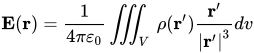
The superposition principle allows for the calculation of the electric field due to a distribution of charge density ${\displaystyle \rho (\mathbf{r})}$. By considering the charge ${\displaystyle \rho ({\mathbf{r}}^{\prime })dv}$ in each small volume of space ${\displaystyle dv}$ at point ${\displaystyle {\mathbf{r}}^{\prime }}$ as a point charge, the resulting electric field, ${\displaystyle d\mathbf{E}(\mathbf{r})}$, at point ${\displaystyle \mathbf{r}}$ can be calculated as $${\displaystyle d\mathbf{E}(\mathbf{r})=\frac{\rho ({\mathbf{r}}^{\prime })}{4\pi {\epsilon }_0}\frac{{\hat{\mathbf{r}}}^{\prime }}{{|{\mathbf{r}}^{\prime }|}^2}dv=\frac{\rho ({\mathbf{r}}^{\prime })}{4\pi {\epsilon }_0}\frac{{\mathbf{r}}^{\prime }}{{|{\mathbf{r}}^{\prime }|}^3}dv}$$ where

• ${\displaystyle {\hat{\mathbf{r}}}^{\prime }}$ is the unit vector pointing from ${\displaystyle {\mathbf{r}}^{\prime }}$ to ${\displaystyle \mathbf{r}}$.
• ${\displaystyle {\mathbf{r}}^{\prime }}$ is the displacement vector from ${\displaystyle {\mathbf{r}}^{\prime }}$ to ${\displaystyle \mathbf{r}}$.

The total field is found by summing the contributions from all the increments of volume by integrating the charge density over the volume ${\displaystyle V}$: $${\displaystyle \mathbf{E}(\mathbf{r})=\frac{1}{4\pi {\epsilon }_0}{\iiint }_V\rho ({\mathbf{r}}^{\prime })\frac{{\mathbf{r}}^{\prime }}{{|{\mathbf{r}}^{\prime }|}^3}dv}$$

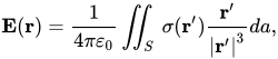
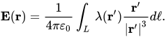
Similar equations follow for a surface charge with surface charge density ${\displaystyle \sigma ({\mathbf{r}}^{\prime })}$ on surface ${\displaystyle S}$ $${\displaystyle \mathbf{E}(\mathbf{r})=\frac{1}{4\pi {\epsilon }_0}{\iint }_S\sigma ({\mathbf{r}}^{\prime })\frac{{\mathbf{r}}^{\prime }}{{|{\mathbf{r}}^{\prime }|}^3}da,}$$ and for line charges with linear charge density ${\displaystyle \lambda ({\mathbf{r}}^{\prime })}$ on line ${\displaystyle L}$ $${\displaystyle \mathbf{E}(\mathbf{r})=\frac{1}{4\pi {\epsilon }_0}{\int }_L\lambda ({\mathbf{r}}^{\prime })\frac{{\mathbf{r}}^{\prime }}{{|{\mathbf{r}}^{\prime }|}^3}d\ell .}$$

Electric potential

Main article: Electric potential

See also: Helmholtz decomposition and Conservative vector field § Irrotational vector fields

If a system is static, such that magnetic fields are not time-varying, then by Faraday's law, the electric field is curl-free. In this case, one can define an electric potential, that is, a function ${\displaystyle \phi }$ such that ${\displaystyle \mathbf{E}=-\mathrm{\nabla }\phi }$. This is analogous to the gravitational potential. The difference between the electric potential at two points in space is called the potential difference (or voltage) between the two points.

In general, however, the electric field cannot be described independently of the magnetic field. Given the magnetic vector potential, A, defined so that ⁠${\displaystyle \mathbf{B}=\mathrm{\nabla }\times \mathbf{A}}$⁠, one can still define an electric potential ${\displaystyle \phi }$ such that: $${\displaystyle \mathbf{E}=-\mathrm{\nabla }\phi -\frac{\mathrm{\partial }\mathbf{A}}{\mathrm{\partial }t},}$$ where ${\displaystyle \mathrm{\nabla }\phi }$ is the gradient of the electric potential and ${\displaystyle \frac{\mathrm{\partial }\mathbf{A}}{\mathrm{\partial }t}}$ is the partial derivative of A with respect to time.

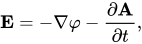
Faraday's law of induction can be recovered by taking the curl of that equation  $${\displaystyle \mathrm{\nabla }\times \mathbf{E}=-\frac{\mathrm{\partial }(\mathrm{\nabla }\times \mathbf{A})}{\mathrm{\partial }t}=-\frac{\mathrm{\partial }\mathbf{B}}{\mathrm{\partial }t},}$$ which justifies, a posteriori, the previous form for E.

Continuous vs. discrete charge representation

Main article: Charge density

The equations of electromagnetism are best described in a continuous description. However, charges are sometimes best described as discrete points; for example, some models may describe electrons as point sources where charge density is infinite on an infinitesimal section of space.

A charge ${\displaystyle q}$ located at ${\displaystyle {\mathbf{r}}_0}$ can be described mathematically as a charge density ⁠${\displaystyle \rho (\mathbf{r})=q\delta (\mathbf{r}-{\mathbf{r}}_0)}$⁠, where the Dirac delta function (in three dimensions) is used. Conversely, a charge distribution can be approximated by many small point charges.

Electrostatic fields

Main article: Electrostatics

Illustration of the electric field surrounding a positive (red) and a negative (blue) charge

Electrostatic fields are electric fields that do not change with time. Such fields are present when systems of charged matter are stationary, or when electric currents are unchanging. In that case, Coulomb's law fully describes the field.

Parallels between electrostatic and gravitational fields

See also: Gravitoelectromagnetism

Coulomb's law, which describes the interaction of electric charges: $${\displaystyle \mathbf{F}=q\left(\frac{Q}{4\pi {\epsilon }_0}\frac{\hat{\mathbf{r}}}{|\mathbf{r}{|}^2}\right)=q\mathbf{E}}$$ is similar to Newton's law of universal gravitation: $${\displaystyle \mathbf{F}=m\left(-GM\frac{\hat{\mathbf{r}}}{|\mathbf{r}{|}^2}\right)=m\mathbf{g}}$$ (where $\hat{\mathbf{r}}=\frac{\mathbf{r}}{\mathbf{|}\mathbf{r}\mathbf{|}}$).

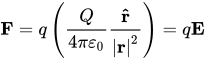
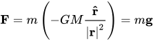
This suggests similarities between the electric field E and the gravitational field g, or their associated potentials. Mass is sometimes called "gravitational charge".

Electrostatic and gravitational forces both are central, conservative and obey an inverse-square law.

Uniform fields

Illustration of the electric field between two parallel conductive plates of finite size (known as a parallel plate capacitor). In the middle of the plates, far from any edges, the electric field is very nearly uniform.

A uniform field is one in which the electric field is constant at every point. It can be approximated by placing two conducting plates parallel to each other and maintaining a voltage (potential difference) between them; it is only an approximation because of boundary effects (near the edge of the planes, the electric field is distorted because the plane does not continue). Assuming infinite planes, the magnitude of the electric field E is: $${\displaystyle E=-\frac{\mathrm{\Delta }V}{d},}$$ where ΔV is the potential difference between the plates and d is the distance separating the plates. The negative sign arises as positive charges repel, so a positive charge will experience a force away from the positively charged plate, in the opposite direction to that in which the voltage increases. In micro- and nano-applications, for instance in relation to semiconductors, a typical magnitude of an electric field is in the order of 10⁶ V⋅m⁻¹, achieved by applying a voltage of the order of 1 volt between conductors spaced 1 μm apart.

Electric field lines

The electric field (lines with arrows) of a charge (+) induces surface charges (red and blue areas) on metal objects due to electrostatic induction.

Main article: field line

A convenient way to plot the electric field that works even for complex electric fields is to use field lines. Here the magnitude and direction of an electric field in a region is represented by a number of non-intersecting curved lines that span the region. If plotted correctly, the direction of the electric field at any given point is represented by the direction of nearby lines while the magnitude is represented by the density of the field lines in that region.

Electric field lines do not intersect. They begin at positive charge (or extend from infinity) and end at negative charge (or extend to infinity). Further the number of field lines from a given charge must be proportional to that charge. Electrostatic fields cannot form closed loops. (See the figure for an example of a complex electric field line diagram made for a positive point charge which induces electrical charge on the surfaces of 3 nearby conductors.

Field lines can only approximately represent the electric field in a given region. (It takes an infinite number of field lines to represent the electric field perfectly.) Nevertheless, these diagrams are useful at illustrating how the electric field changes over a given region.

Electromagnetic fields

Main article: Electromagnetic field

Electromagnetic fields are electric and magnetic fields, which may change with time, for instance when charges are in motion. Moving charges produce a magnetic field in accordance with Ampère's circuital law (with Maxwell's addition), which, along with Maxwell's other equations, defines the magnetic field, ${\displaystyle \mathbf{B}}$, in terms of its curl: $${\displaystyle \mathrm{\nabla }\times \mathbf{B}={\mu }_0\left(\mathbf{J}+{\epsilon }_0\frac{\mathrm{\partial }\mathbf{E}}{\mathrm{\partial }t}\right),}$$ where ${\displaystyle \mathbf{J}}$ is the current density, ${\displaystyle {\mu }_0}$ is the vacuum permeability, and ${\displaystyle {\epsilon }_0}$ is the vacuum permittivity.

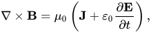
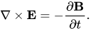
Both the electric current density and the partial derivative of the electric field with respect to time, contribute to the curl of the magnetic field. In addition, the Maxwell–Faraday equation states $${\displaystyle \mathrm{\nabla }\times \mathbf{E}=-\frac{\mathrm{\partial }\mathbf{B}}{\mathrm{\partial }t}.}$$ These represent two of Maxwell's four equations and they intricately link the electric and magnetic fields together, resulting in the electromagnetic field. The equations represent a set of four coupled multi-dimensional partial differential equations which, when solved for a system, describe the combined behavior of the electromagnetic fields. In general, the force experienced by a test charge in an electromagnetic field is given by the Lorentz force law: $${\displaystyle \mathbf{F}=q\mathbf{E}+q\mathbf{v}\times \mathbf{B}.}$$

Energy in the electric field

The total energy per unit volume stored by the electromagnetic field is $${\displaystyle u_{\text{EM}}=\frac{\epsilon }{2}|\mathbf{E}{|}^2+\frac{1}{2\mu }|\mathbf{B}{|}^2}$$ where ε is the permittivity of the medium in which the field exists, ${\displaystyle \mu }$ its magnetic permeability, and E and B are the electric and magnetic field vectors.

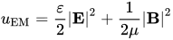
As E and B fields are coupled, it would be misleading to split this expression into "electric" and "magnetic" contributions. In particular, an electrostatic field in any given frame of reference in general transforms into a field with a magnetic component in a relatively moving frame. Accordingly, decomposing the electromagnetic field into an electric and magnetic component is frame-specific, and similarly for the associated energy.

The total energy U_EM stored in the electromagnetic field in a given volume V is $${\displaystyle U_{\text{EM}}=\frac{1}{2}{\int }_V\left(\epsilon |\mathbf{E}{|}^2+\frac{1}{\mu }|\mathbf{B}{|}^2\right)dV.}$$

Electric displacement field

Main article: electric displacement field

Definitive equation of vector fields

See also: List of electromagnetism equations

In the presence of matter, it is helpful to extend the notion of the electric field into three vector fields: $${\displaystyle \mathbf{D}={\epsilon }_0\mathbf{E}+\mathbf{P}}$$ where P is the electric polarization – the volume density of electric dipole moments, and D is the electric displacement field. Since E and P are defined separately, this equation can be used to define D. The physical interpretation of D is not as clear as E (effectively the field applied to the material) or P (induced field due to the dipoles in the material), but still serves as a convenient mathematical simplification, since Maxwell's equations can be simplified in terms of free charges and currents.

Constitutive relation

Main article: Constitutive equation

The E and D fields are related by the permittivity of the material, ε.

For linear, homogeneous, isotropic materials E and D are proportional and constant throughout the region, there is no position dependence: $${\displaystyle \mathbf{D}(\mathbf{r})=\epsilon \mathbf{E}(\mathbf{r}).}$$

For inhomogeneous materials, there is a position dependence throughout the material: $${\displaystyle \mathbf{D}(\mathbf{r})=\epsilon (\mathbf{r})\mathbf{E}(\mathbf{r})}$$

For anisotropic materials the E and D fields are not parallel, and so E and D are related by the permittivity tensor (a 2nd order tensor field), in component form: $${\displaystyle D_i={\epsilon }_{ij}{E}_j}$$

For non-linear media, E and D are not proportional. Materials can have varying extents of linearity, homogeneity and isotropy.

Relativistic effects on electric field

Point charge in uniform motion

The invariance of the form of Maxwell's equations under Lorentz transformation can be used to derive the electric field of a uniformly moving point charge. The charge of a particle is considered frame invariant, as supported by experimental evidence. Alternatively the electric field of uniformly moving point charges can be derived from the Lorentz transformation of four-force experienced by test charges in the source's rest frame given by Coulomb's law and assigning electric field and magnetic field by their definition given by the form of Lorentz force. However the following equation is only applicable when no acceleration is involved in the particle's history where Coulomb's law can be considered or symmetry arguments can be used for solving Maxwell's equations in a simple manner. The electric field of such a uniformly moving point charge is hence given by: $${\displaystyle \mathbf{E}=\frac{q}{4\pi {\epsilon }_0{r}^3}\frac{1-{\beta }^2}{(1-{\beta }^2{\sin }^2\theta {)}^{3/2}}\mathbf{r},}$$ where ${\displaystyle q}$ is the charge of the point source, ${\displaystyle \mathbf{r}}$ is the position vector from the point source to the point in space, ${\displaystyle \beta }$ is the ratio of observed speed of the charge particle to the speed of light and ${\displaystyle \theta }$ is the angle between ${\displaystyle \mathbf{r}}$ and the observed velocity of the charged particle.

The above equation reduces to that given by Coulomb's law for non-relativistic speeds of the point charge. Spherical symmetry is not satisfied due to breaking of symmetry in the problem by specification of direction of velocity for calculation of field. To illustrate this, field lines of moving charges are sometimes represented as unequally spaced radial lines which would appear equally spaced in a co-moving reference frame.

Propagation of disturbances in electric fields

See also: Paradox of radiation of charged particles in a gravitational field

Special theory of relativity imposes the principle of locality, that requires cause and effect to be time-like separated events where the causal efficacy does not travel faster than the speed of light. Maxwell's laws are found to confirm to this view since the general solutions of fields are given in terms of retarded time which indicate that electromagnetic disturbances travel at the speed of light. Advanced time, which also provides a solution for Maxwell's law are ignored as an unphysical solution. For the motion of a charged particle, considering for example the case of a moving particle with the above described electric field coming to an abrupt stop, the electric fields at points far from it do not immediately revert to that classically given for a stationary charge. On stopping, the field around the stationary points begin to revert to the expected state and this effect propagates outwards at the speed of light while the electric field lines far away from this will continue to point radially towards an assumed moving charge. This virtual particle will never be outside the range of propagation of the disturbance in electromagnetic field, since charged particles are restricted to have speeds slower than that of light, which makes it impossible to construct a Gaussian surface in this region that violates Gauss's law. Another technical difficulty that supports this is that charged particles travelling faster than or equal to speed of light no longer have a unique retarded time. Since electric field lines are continuous, an electromagnetic pulse of radiation is generated that connects at the boundary of this disturbance travelling outwards at the speed of light. In general, any accelerating point charge radiates electromagnetic waves however, non-radiating acceleration is possible in a systems of charges.

Arbitrarily moving point charge

See also: Jefimenko's equations § Heaviside–Feynman formula

For arbitrarily moving point charges, propagation of potential fields such as Lorenz gauge fields at the speed of light needs to be accounted for by using Liénard–Wiechert potential. Since the potentials satisfy Maxwell's equations, the fields derived for point charge also satisfy Maxwell's equations. The electric field is expressed as: $${\displaystyle \mathbf{E}(\mathbf{r},\mathbf{t})=\frac{q}{4\pi {\epsilon }_0}{\left(\frac{\left({\mathbf{n}}_s-{\mathit{\beta }}_s\right)}{{\gamma }^2{\left(1-{\mathbf{n}}_s\cdot {\mathit{\beta }}_s\right)}^3{\left|\mathbf{r}-{\mathbf{r}}_s\right|}^2}+\frac{{\mathbf{n}}_s\times \left(\left({\mathbf{n}}_s-{\mathit{\beta }}_s\right)\times \dot{{\mathit{\beta }}_s}\right)}{c{\left(1-{\mathbf{n}}_s\cdot {\mathit{\beta }}_s\right)}^3\left|\mathbf{r}-{\mathbf{r}}_s\right|}\right)}_{t=t_r}}$$ where ${\displaystyle q}$ is the charge of the point source, $t_r$ is retarded time or the time at which the source's contribution of the electric field originated, $r_s(t)$ is the position vector of the particle, ${\mathbf{n}}_s(\mathbf{r},t)$ is a unit vector pointing from charged particle to the point in space, ${\mathit{\beta }}_s(t)$ is the velocity of the particle divided by the speed of light, and $\gamma (t)$ is the corresponding Lorentz factor. The retarded time is given as solution of: $${\displaystyle t_r=t-\frac{|\mathbf{r}-{\mathbf{r}}_s(t_r)|}{c}}$$

The uniqueness of solution for $t_r$ for given ${\displaystyle t}$, ${\displaystyle \mathbf{r}}$ and ${\displaystyle r_s(t)}$ is valid for charged particles moving slower than speed of light. Electromagnetic radiation of accelerating charges is known to be caused by the acceleration dependent term in the electric field from which relativistic correction for Larmor formula is obtained.

There exist yet another set of solutions for Maxwell's equation of the same form but for advanced time $t_a$ instead of retarded time given as a solution of:

$${\displaystyle t_a=t+\frac{\left|\mathbf{r}-{\mathbf{r}}_s(t_a)\right|}{c}}$$

Since the physical interpretation of this indicates that the electric field at a point is governed by the particle's state at a point of time in the future, it is considered as an unphysical solution and hence neglected. However, there have been theories exploring the advanced time solutions of Maxwell's equations, such as Feynman Wheeler absorber theory.

The above equation, although consistent with that of uniformly moving point charges as well as its non-relativistic limit, are not corrected for quantum-mechanical effects.

Multiverse

From Wikipedia, the free encyclopedia

https://en.wikipedia.org/wiki/Multiverse

The multiverse is the hypothetical set of all universes. Together, these universes are presumed to comprise everything that exists: the entirety of space, time, matter, energy, information, and the physical laws and constants that describe them. The different universes within the multiverse are called "parallel universes", "flat universes", "other universes", "alternate universes", "multiple universes", "plane universes", "parent and child universes", "many universes", or "many worlds". One common assumption is that the multiverse is a "patchwork quilt of separate universes all bound by the same laws of physics."

The concept of multiple universes, or a multiverse, has been discussed throughout history. It has evolved and has been debated in various fields, including cosmology, physics, and philosophy. Some physicists have argued that the multiverse is a philosophical notion rather than a scientific hypothesis, as it cannot be empirically falsified. In recent years, there have been proponents and skeptics of multiverse theories within the physics community. Although some scientists have analyzed data in search of evidence for other universes, no statistically significant evidence has been found. Critics argue that the multiverse concept lacks testability and falsifiability, which are essential for scientific inquiry, and that it raises unresolved metaphysical issues.

Max Tegmark and Brian Greene have proposed different classification schemes for multiverses and universes. Tegmark's four-level classification consists of Level I: an extension of our universe, Level II: universes with different physical constants, Level III: many-worlds interpretation of quantum mechanics, and Level IV: ultimate ensemble. Brian Greene's nine types of multiverses include quilted, inflationary, brane, cyclic, landscape, quantum, holographic, simulated, and ultimate. The ideas explore various dimensions of space, physical laws, and mathematical structures to explain the existence and interactions of multiple universes. Some other multiverse concepts include twin-world models, cyclic theories, M-theory, and black-hole cosmology.

The anthropic principle suggests that the existence of a multitude of universes, each with different physical laws, could explain the asserted appearance of fine-tuning of our own universe for conscious life. The weak anthropic principle posits that we exist in one of the few universes that support life. Debates around Occam's razor and the simplicity of the multiverse versus a single universe arise, with proponents like Max Tegmark arguing that the multiverse is simpler and more elegant. The many-worlds interpretation of quantum mechanics and modal realism, the belief that all possible worlds exist and are as real as our world, are also subjects of debate in the context of the anthropic principle.

History of the concept

According to some, the idea of infinite worlds was first suggested by the pre-Socratic Greek philosopher Anaximander in the sixth century BCE. However, there is debate as to whether he believed in multiple worlds, and if he did, whether those worlds were co-existent or successive.

Ancient Indian thinkers, both Hindu and Buddhist, postulated multiple worlds/realms/universes.

The first figures to whom historians can definitively attribute the concept of innumerable worlds are the Ancient Greek Atomists, beginning with Leucippus and Democritus in the 5th century BCE, followed by Epicurus (341–270 BCE) and the Roman Epicurean Lucretius (1st century BCE). In the third century BCE, the philosopher Chrysippus suggested that the world eternally expired and regenerated, effectively suggesting the existence of multiple universes across time. The concept of multiple universes became more defined in the Middle Ages. In the Renaissance, Giordano Bruno (1548–1600) expressed the concept of infinite worlds.

The American philosopher and psychologist William James used the term "multiverse" in 1895, but in a different context.

The concept first appeared in the modern scientific context in the course of the debate between Boltzmann and Zermelo in 1895.

In Dublin in 1952, Erwin Schrödinger gave a lecture in which he jocularly warned his audience that what he was about to say might "seem lunatic". He said that when his equations seemed to describe several different histories, these were "not alternatives, but all really happen simultaneously". This sort of duality is called "superposition".

Search for evidence

In the 1990s, after recent works of fiction about the concept gained popularity, scientific discussions about the multiverse and journal articles about it gained prominence.

Around 2010, scientists such as Stephen M. Feeney analyzed Wilkinson Microwave Anisotropy Probe (WMAP) data and claimed to find evidence suggesting that this universe collided with other (parallel) universes in the distant past. However, a more thorough analysis of data from the WMAP and from the Planck satellite, which has a resolution three times higher than WMAP, did not reveal any statistically significant evidence of such a bubble universe collision. In addition, there was no evidence of any gravitational pull of other universes on ours.

In 2015, an astrophysicist may have found evidence of alternate or parallel universes by looking back in time to a time immediately after the Big Bang, although it is still a matter of debate among physicists. Dr. Ranga-Ram Chary, after analyzing the cosmic radiation spectrum, found a signal 4,500 times brighter than it should have been, based on the number of protons and electrons scientists believe existed in the very early universe. This signal—an emission line that arose from the formation of atoms during the era of recombination—is more consistent with a universe whose ratio of matter particles to photons is about 65 times greater than our own. There is a 30% chance that this signal is noise, and not really a signal at all; however, it is also possible that it exists because a parallel universe dumped some of its matter particles into our universe. If additional protons and electrons had been added to our universe during recombination, more atoms would have formed, more photons would have been emitted during their formation, and the signature line that arose from all of these emissions would be greatly enhanced. Chary said:

Many other regions beyond our observable universe would exist with each such region governed by a different set of physical parameters than the ones we have measured for our universe.

— Ranga-Ram Chary, USA Today

Chary also noted:

Unusual claims like evidence for alternate universes require a very high burden of proof.

— Ranga-Ram Chary, "Universe Today"

The signature that Chary has isolated may be a consequence of incoming light from distant galaxies, or even from clouds of dust surrounding our own galaxy.

Proponents and skeptics

Modern proponents of one or more of the multiverse hypotheses include Lee Smolin, Don Page, Brian Greene, Max Tegmark, Alan Guth, Andrei Linde, Michio Kaku, David Deutsch, Leonard Susskind, Alexander Vilenkin, Yasunori Nomura, Raj Pathria, Laura Mersini-Houghton, Neil deGrasse Tyson, Sean Carroll and Stephen Hawking.

Scientists who are generally skeptical of the concept of a multiverse or popular multiverse hypotheses include Sabine Hossenfelder, David Gross, Paul Steinhardt, Anna Ijjas, Abraham Loeb, David Spergel, Neil Turok, Viatcheslav Mukhanov, Michael S. Turner, Roger Penrose, George Ellis, Joe Silk, Carlo Rovelli, Adam Frank, Marcelo Gleiser, Jim Baggott and Paul Davies.

Arguments against multiverse hypotheses

In his 2003 New York Times opinion piece, "A Brief History of the Multiverse", author and cosmologist Paul Davies offered a variety of arguments that multiverse hypotheses are non-scientific:

For a start, how is the existence of the other universes to be tested? To be sure, all cosmologists accept that there are some regions of the universe that lie beyond the reach of our telescopes, but somewhere on the slippery slope between that and the idea that there is an infinite number of universes, credibility reaches a limit. As one slips down that slope, more and more must be accepted on faith, and less and less is open to scientific verification. Extreme multiverse explanations are therefore reminiscent of theological discussions. Indeed, invoking an infinity of unseen universes to explain the unusual features of the one we do see is just as ad hoc as invoking an unseen Creator. The multiverse theory may be dressed up in scientific language, but in essence, it requires the same leap of faith.

— Paul Davies, "A Brief History of the Multiverse", The New York Times

George Ellis, writing in August 2011, provided a criticism of the multiverse, and pointed out that it is not a traditional scientific theory. He accepts that the multiverse is thought to exist far beyond the cosmological horizon. He emphasized that it is theorized to be so far away that it is unlikely any evidence will ever be found. Ellis also explained that some theorists do not believe the lack of empirical testability and falsifiability is a major concern, but he is opposed to that line of thinking:

Many physicists who talk about the multiverse, especially advocates of the string landscape, do not care much about parallel universes per se. For them, objections to the multiverse as a concept are unimportant. Their theories live or die based on internal consistency and, one hopes, eventual laboratory testing.

Ellis says that scientists have proposed the idea of the multiverse as a way of explaining the nature of existence. He points out that it ultimately leaves those questions unresolved because it is a metaphysical issue that cannot be resolved by empirical science. He argues that observational testing is at the core of science and should not be abandoned:

As skeptical as I am, I think the contemplation of the multiverse is an excellent opportunity to reflect on the nature of science and on the ultimate nature of existence: why we are here. ... In looking at this concept, we need an open mind, though not too open. It is a delicate path to tread. Parallel universes may or may not exist; the case is unproved. We are going to have to live with that uncertainty. Nothing is wrong with scientifically based philosophical speculation, which is what multiverse proposals are. But we should name it for what it is.

— George Ellis, "Does the Multiverse Really Exist?", Scientific American

Philosopher Philip Goff argues that the inference of a multiverse to explain the apparent fine-tuning of the universe is an example of Inverse Gambler's Fallacy.

Stoeger, Ellis, and Kircher note that in a true multiverse theory, "the universes are then completely disjoint and nothing that happens in any one of them is causally linked to what happens in any other one. This lack of any causal connection in such multiverses really places them beyond any scientific support".

In May 2020, in a Forbes blog post, astrophysicist Ethan Siegel expressed criticism of the claim of results from the Antarctic Impulsive Transient Antenna providing evidence for the multiverse, commenting that parallel universes would have to remain a science fiction dream for the time being.

Scientific American contributor John Horgan also argues against the idea of a multiverse, claiming that they are "bad for science."

Types

Max Tegmark and Brian Greene have devised classification schemes for the various theoretical types of multiverses and universes that they might comprise.

Max Tegmark's four levels

Cosmologist Max Tegmark has provided a taxonomy of universes beyond the familiar observable universe. The four levels of Tegmark's classification are arranged such that subsequent levels can be understood to encompass and expand upon previous levels. They are briefly described below.

Level I: An extension of our universe

A prediction of cosmic inflation is the existence of an infinite ergodic universe, which, being infinite, must contain Hubble volumes realizing all initial conditions.

Accordingly, an infinite universe will contain an infinite number of Hubble volumes, all having the same physical laws and physical constants. In regard to configurations such as the distribution of matter, almost all will differ from our Hubble volume. However, because there are infinitely many, far beyond the cosmological horizon, there will eventually be Hubble volumes with similar, and even identical, configurations. Tegmark estimates that an identical volume to ours should be about 10¹⁰¹¹⁵ meters away from us.

Given infinite space, there would be an infinite number of Hubble volumes identical to ours in the universe. This follows directly from the cosmological principle, wherein it is assumed that our Hubble volume is not special or unique.

Level II: Universes with different physical constants

In the eternal inflation theory, which is a variant of the cosmic inflation theory, the multiverse or space as a whole is stretching and will continue doing so forever, but some regions of space stop stretching and form distinct bubbles (like gas pockets in a loaf of rising bread). Such bubbles are embryonic level I multiverses.

Different bubbles may experience different spontaneous symmetry breaking, which results in different properties, such as different physical constants.

Level II also includes John Archibald Wheeler's oscillatory universe theory and Lee Smolin's fecund universes theory.

Level III: Many-worlds interpretation of quantum mechanics

Schrödinger's cat in the many-worlds interpretation, where a branching of the universe occurs through a superposition of two quantum mechanical states

Hugh Everett III's many-worlds interpretation (MWI) is one of several mainstream interpretations of quantum mechanics.

In brief, one aspect of quantum mechanics is that certain observations cannot be predicted absolutely. Instead, there is a range of possible observations, each with a different probability. According to the MWI, each of these possible observations corresponds to a different "world" within the universal wave function, with each world as real as ours. Suppose a six-sided die is thrown and that the result of the throw corresponds to observable quantum mechanics. All six possible ways the die can fall correspond to six different worlds. In the case of the Schrödinger's cat thought experiment, both outcomes would be "real" in at least one "world".

Tegmark argues that a Level III multiverse does not contain more possibilities in the Hubble volume than a Level I or Level II multiverse. In effect, all the different worlds created by "splits" in a Level III multiverse with the same physical constants can be found in some Hubble volume in a Level I multiverse. Tegmark writes that, "The only difference between Level I and Level III is where your doppelgängers reside. In Level I they live elsewhere in good old three-dimensional space. In Level III they live on another quantum branch in infinite-dimensional Hilbert space."

Similarly, all Level II bubble universes with different physical constants can, in effect, be found as "worlds" created by "splits" at the moment of spontaneous symmetry breaking in a Level III multiverse. According to Yasunori Nomura, Raphael Bousso, and Leonard Susskind, this is because global spacetime appearing in the (eternally) inflating multiverse is a redundant concept. This implies that the multiverses of Levels I, II, and III are, in fact, the same thing. This hypothesis is referred to as "Multiverse = Quantum Many Worlds". According to Yasunori Nomura, this quantum multiverse is static, and time is a simple illusion.

Another version of the many-worlds idea is H. Dieter Zeh's many-minds interpretation.

Level IV: Ultimate ensemble

The ultimate mathematical universe hypothesis is Tegmark's own hypothesis.

This level considers all universes to be equally real which can be described by different mathematical structures.

Tegmark writes:

Abstract mathematics is so general that any Theory Of Everything (TOE) which is definable in purely formal terms (independent of vague human terminology) is also a mathematical structure. For instance, a TOE involving a set of different types of entities (denoted by words, say) and relations between them (denoted by additional words) is nothing but what mathematicians call a set-theoretical model, and one can generally find a formal system that it is a model of.

He argues that this "implies that any conceivable parallel universe theory can be described at Level IV" and "subsumes all other ensembles, therefore brings closure to the hierarchy of multiverses, and there cannot be, say, a Level V."

Jürgen Schmidhuber, however, says that the set of mathematical structures is not even well-defined and that it admits only universe representations describable by constructive mathematics—that is, computer programs.

Schmidhuber explicitly includes universe representations describable by non-halting programs whose output bits converge after a finite time, although the convergence time itself may not be predictable by a halting program, due to the undecidability of the halting problem. He also explicitly discusses the more restricted ensemble of quickly computable universes.

Brian Greene's nine types

The American theoretical physicist and string theorist Brian Greene discussed nine types of multiverses:

Quilted

The quilted multiverse works only in an infinite universe. With an infinite amount of space, every possible event will occur an infinite number of times. However, the speed of light prevents us from being aware of these other identical areas.

Inflationary

The inflationary multiverse is composed of various pockets in which inflation fields collapse and form new universes.

Duration: 10 seconds.0:10

Animation showing the multiple brane universes in the bulk

Brane

The brane multiverse version postulates that our entire universe exists on a membrane (brane) which floats in a higher dimension or "bulk". In this bulk, there are other membranes with their own universes. These universes can interact with one another, and when they collide, the violence and energy produced is more than enough to give rise to a Big Bang. The branes float or drift near each other in the bulk, and every few trillion years, attracted by gravity or some other force we do not understand, collide and bang into each other. This repeated contact gives rise to multiple or "cyclic" Big Bangs. This particular hypothesis falls under the string theory umbrella as it requires extra spatial dimensions.

Cosmos animation of a cyclic universe

Cyclic

The cyclic multiverse has multiple branes that have collided, causing Big Bangs. The universes bounce back and pass through time until they are pulled back together and again collide, destroying the old contents and creating them anew.

Landscape

The landscape multiverse relies on string theory's Calabi–Yau spaces. Quantum fluctuations drop the shapes to a lower energy level, creating a pocket with a set of laws different from that of the surrounding space.

Quantum

The quantum multiverse creates a new universe when a diversion in events occurs, as in the real-worlds variant of the many-worlds interpretation of quantum mechanics.

Holographic

The holographic multiverse is derived from the theory that the surface area of a space can encode the contents of the volume of the region.

Simulated

The simulated multiverse exists on complex computer systems that simulate entire universes. A related hypothesis, as put forward as a possibility by astronomer Avi Loeb, is that universes may be creatable in laboratories of advanced technological civilizations who have a theory of everything. Other related hypotheses include brain in a vat-type scenarios where the perceived universe is either simulated in a low-resource way or not perceived directly by the virtual/simulated inhabitant species.

Ultimate

The ultimate multiverse contains every mathematically possible universe under different laws of physics.

Twin-world models

Concept of a twin universe, with the beginning of time in the middle

There are models of two related universes that e.g. attempt to explain the baryon asymmetry – why there was more matter than antimatter at the beginning – with a mirror anti-universe. One two-universe cosmological model could explain the Hubble constant (H₀) tension via interactions between the two worlds. The "mirror world" would contain copies of all existing fundamental particles. Another twin/pair-world or "bi-world" cosmology is shown to theoretically be able to solve the cosmological constant (Λ) problem, closely related to dark energy: two interacting worlds with a large Λ each could result in a small shared effective Λ.

Cyclic theories

Main article: Cyclic model

In several theories, there is a series of, in some cases infinite, self-sustaining cycles – typically a series of Big Crunches (or Big Bounces). However, the respective universes do not exist at once but are forming or following in a logical order or sequence, with key natural constituents potentially varying between universes (see § Anthropic principle).

M-theory

See also: Introduction to M-theory, M-theory, Brane cosmology, and String theory landscape

A multiverse of a somewhat different kind has been envisaged within string theory and its higher-dimensional extension, M-theory.

These theories require the presence of 10 or 11 spacetime dimensions, respectively. The extra six or seven dimensions may either be compactified on a very small scale, or our universe may simply be localized on a dynamical (3+1)-dimensional object, a D3-brane. This opens up the possibility that there are other branes which could support other universes.

Black-hole cosmology

Main article: Black-hole cosmology

Black-hole cosmology is a cosmological model in which the observable universe is the interior of a black hole existing as one of possibly many universes inside a larger universe. This includes the theory of white holes, which are on the opposite side of space-time.

Anthropic principle

Main article: Anthropic principle

The concept of other universes has been proposed to explain how our own universe appears to be fine-tuned for conscious life as we experience it.

If there were a large (possibly infinite) number of universes, each with possibly different physical laws (or different fundamental physical constants), then some of these universes (even if very few) would have the combination of laws and fundamental parameters that are suitable for the development of matter, astronomical structures, elemental diversity, stars, and planets that can exist long enough for life to emerge and evolve.

The weak anthropic principle could then be applied to conclude that we (as conscious beings) would only exist in one of those few universes that happened to be finely tuned, permitting the existence of life with developed consciousness. Thus, while the probability might be extremely small that any particular universe would have the requisite conditions for life (as we understand life), those conditions do not require intelligent design as an explanation for the conditions in the Universe that promote our existence in it.

An early form of this reasoning is evident in Arthur Schopenhauer's 1844 work "Von der Nichtigkeit und dem Leiden des Lebens", where he argues that our world must be the worst of all possible worlds, because if it were significantly worse in any respect it could not continue to exist.

Occam's razor

Proponents and critics disagree about how to apply Occam's razor. Critics argue that to postulate an almost infinite number of unobservable universes, just to explain our own universe, is contrary to Occam's razor. However, proponents argue that in terms of Kolmogorov complexity the proposed multiverse is simpler than a single idiosyncratic universe.

For example, multiverse proponent Max Tegmark argues:

[A]n entire ensemble is often much simpler than one of its members. This principle can be stated more formally using the notion of algorithmic information content. The algorithmic information content in a number is, roughly speaking, the length of the shortest computer program that will produce that number as output. For example, consider the set of all integers. Which is simpler, the whole set or just one number? Naively, you might think that a single number is simpler, but the entire set can be generated by quite a trivial computer program, whereas a single number can be hugely long. Therefore, the whole set is actually simpler... (Similarly), the higher-level multiverses are simpler. Going from our universe to the Level I multiverse eliminates the need to specify initial conditions, upgrading to Level II eliminates the need to specify physical constants, and the Level IV multiverse eliminates the need to specify anything at all... A common feature of all four multiverse levels is that the simplest and arguably most elegant theory involves parallel universes by default. To deny the existence of those universes, one needs to complicate the theory by adding experimentally unsupported processes and ad hoc postulates: finite space, wave function collapse and ontological asymmetry. Our judgment therefore comes down to which we find more wasteful and inelegant: many worlds or many words. Perhaps we will gradually get used to the weird ways of our cosmos and find its strangeness to be part of its charm.

— Max Tegmark

Possible worlds and real worlds

In any given set of possible universes – e.g. in terms of histories or variables of nature – not all may be ever realized, and some may be realized many times. For example, over infinite time there could, in some potential theories, be infinite universes, but only a small or relatively small real number of universes where humanity could exist and only one where it ever does exist (with a unique history). It has been suggested that a universe that "contains life, in the form it has on Earth, is in a certain sense radically non-ergodic, in that the vast majority of possible organisms will never be realized". On the other hand, some scientists, theories and popular works conceive of a multiverse in which the universes are so similar that humanity exists in many equally real separate universes but with varying histories.

There is a debate about whether the other worlds are real in the many-worlds interpretation (MWI) of quantum mechanics. In Quantum Darwinism one does not need to adopt a MWI in which all of the branches are equally real.

Modal realism

Possible worlds are a way of explaining probability and hypothetical statements. Some philosophers, such as David Lewis, posit that all possible worlds exist and that they are just as real as the world we live in. This position is known as modal realism.