Probability density function

From Wikipedia, the free encyclopedia

https://en.wikipedia.org/wiki/Probability_density_function 

Box plot and probability density function of a normal distribution N(0, σ²).

Geometric visualisation of the mode, median and mean of an arbitrary unimodal probability density function.

In probability theory, a probability density function (PDF), density function, or simply density of an absolutely continuous random variable, is a function whose value at any given point in the sample space (the set of possible values taken by the random variable) can be interpreted as providing a "relative probability" that the value of the random variable would be equal to that point. Probability density is the probability per unit length, in other words. The (absolute) probability for a continuous random variable to take on any particular value is zero. Therefore, the value of the PDF at two different samples can be used to infer, in any particular draw of the random variable, how much more likely it is that the random variable would be close to one point compared to the other.

More precisely, the PDF is used to specify the probability of the random variable falling within a particular range of values, as opposed to taking on any one value. This probability is given by the integral of a continuous variable's PDF over that range, where the integral is the nonnegative area under the density function between the lowest and greatest values of the range. The PDF is nonnegative everywhere, and the area under the entire curve is equal to one, such that the probability of the random variable falling within the set of possible values is 100%.

The terms probability distribution function and probability function can also denote the probability density function. However, this use is not standard among probabilists and statisticians. In other sources, "probability distribution function" may be used when the probability distribution is defined as a function over general sets of values or it may refer to the cumulative distribution function (CDF), or it may be a probability mass function (PMF) rather than the density. Density function itself is also used for the probability mass function, leading to further confusion. In general the PMF is used in the context of discrete random variables (random variables that take values on a countable set), while the PDF is used in the context of continuous random variables. Both PMF and PDF are fundamental concepts in statistical inference.

Example

Examples of four continuous probability density functions.

Suppose bacteria of a certain species typically live 20 to 30 hours. The probability that a bacterium lives exactly 5 hours is equal to zero (we are talking about an idealized real-valued variable, not the recorded observation). A lot of bacteria live for approximately 5 hours, but there is no chance that any given bacterium dies at exactly 5.00... hours (measured with infinite precision). However, the probability that the bacterium dies between 5 hours and 5.01 hours is quantifiable. Suppose the answer is 0.02 (i.e., 2%). Then, the probability that the bacterium dies between 5 hours and 5.001 hours should be about 0.002, since this time interval is one-tenth as long as the previous. The probability that the bacterium dies between 5 hours and 5.0001 hours should be about 0.0002, and so on.

In this example, the ratio (probability of dying during an interval) / (duration of the interval) is approximately constant, and equal to 2 per hour (or 2 hour⁻¹). For example, there is 0.02 probability of dying in the 0.01-hour interval between 5 and 5.01 hours, and (0.02 probability / 0.01 hours) = 2 hour⁻¹. This quantity 2 hour⁻¹ is called the probability density for dying at around 5 hours. Therefore, the probability that the bacterium dies at 5 hours can be written as (2 hour⁻¹) dt. This is the probability that the bacterium dies within an infinitesimal window of time around 5 hours, where dt is the duration of this window. For example, the probability that it lives longer than 5 hours, but shorter than (5 hours + 1 nanosecond), is (2 hour⁻¹)×(1 nanosecond) ≈ 6×10⁻¹³ (using the unit conversion 3.6×10¹² nanoseconds = 1 hour).

There is a probability density function f with f(5 hours) = 2 hour⁻¹. The integral of f over any window of time (not only infinitesimal windows but also large windows) is the probability that the bacterium dies in that window.

Absolutely continuous univariate distributions

A probability density function is most commonly associated with absolutely continuous univariate distributions. A random variable ${\displaystyle X}$ has density ${\displaystyle f_X}$, where ${\displaystyle f_X}$ is a non-negative Lebesgue-integrable function, if: $${\displaystyle Pr[a\le X\le b]={\int }_a^b{f}_X(x)dx.}$$

Hence, if ${\displaystyle F_X}$ is the cumulative distribution function of ${\displaystyle X}$, then: $${\displaystyle F_X(x)={\int }_{-\mathrm{\infty }}^x{f}_X(u)du,}$$ and (if ${\displaystyle F_X}$ is differentiable at ${\displaystyle x}$) $${\displaystyle f_X(x)=\frac{d}{dx}{F}_X(x).}$$

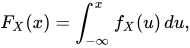
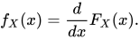
Intuitively, one can think of ${\displaystyle f_X(x)dx}$ as being the probability of ${\displaystyle X}$ falling within the infinitesimal interval ${\displaystyle [x,x+dx]}$.

Formal definition

(This definition may be extended to any probability distribution using the measure-theoretic definition of probability.)

A random variable ${\displaystyle X}$ with values in a measurable space ${\displaystyle (\mathcal{X},\mathcal{A})}$ (usually ${\displaystyle {\mathbb{R}}^n}$ with the Borel sets as measurable subsets) has as probability distribution the pushforward measure X_∗P on ${\displaystyle (\mathcal{X},\mathcal{A})}$: the density of ${\displaystyle X}$ with respect to a reference measure ${\displaystyle \mu }$ on ${\displaystyle (\mathcal{X},\mathcal{A})}$ is the Radon–Nikodym derivative: $${\displaystyle f=\frac{d{X}_{\ast }P}{d\mu }.}$$

That is, f is any measurable function with the property that: $${\displaystyle Pr[X\in A]={\int }_{X^{-1}A}dP={\int }_{A}fd\mu }$$ for any measurable set ${\displaystyle A\in \mathcal{A}.}$

Discussion

In the continuous univariate case above, the reference measure is the Lebesgue measure. The probability mass function of a discrete random variable is the density with respect to the counting measure over the sample space (usually the set of integers, or some subset thereof).

It is not possible to define a density with reference to an arbitrary measure (e.g. one can not choose the counting measure as a reference for a continuous random variable). Furthermore, when it does exist, the density is almost unique, meaning that any two such densities coincide almost everywhere.

Further details

Unlike a probability, a probability density function can take on values greater than one; for example, the continuous uniform distribution on the interval [0, 1/2] has probability density f(x) = 2 for 0 ≤ x ≤ 1/2 and f(x) = 0 elsewhere.

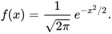
The standard normal distribution has probability density$${\displaystyle f(x)=\frac{1}{\sqrt{2\pi }}{e}^{-x^2/2}.}$$

If a random variable X is given and its distribution admits a probability density function f, then the expected value of X (if the expected value exists) can be calculated as$${\displaystyle \mathrm{E}[X]={\int }_{-\mathrm{\infty }}^{\mathrm{\infty }}xf(x)dx.}$$

Not every probability distribution has a density function: the distributions of discrete random variables do not; nor does the Cantor distribution, even though it has no discrete component, i.e., does not assign positive probability to any individual point.

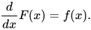
A distribution has a density function if its cumulative distribution function F(x) is absolutely continuous. In this case: F is almost everywhere differentiable, and its derivative can be used as probability density:$${\displaystyle \frac{d}{dx}F(x)=f(x).}$$

If a probability distribution admits a density, then the probability of every one-point set {a} is zero; the same holds for finite and countable sets.

Two probability densities f and g represent the same probability distribution precisely if they differ only on a set of Lebesgue measure zero.

In the field of statistical physics, a non-formal reformulation of the relation above between the derivative of the cumulative distribution function and the probability density function is generally used as the definition of the probability density function. This alternate definition is the following:

If dt is an infinitely small number, the probability that X is included within the interval (t, t + dt) is equal to f(t) dt, or: $${\displaystyle Pr(t<X<t+dt)=f(t)dt.}$$

Link between discrete and continuous distributions

It is possible to represent certain discrete random variables as well as random variables involving both a continuous and a discrete part with a generalized probability density function using the Dirac delta function. (This is not possible with a probability density function in the sense defined above, it may be done with a distribution.) For example, consider a binary discrete random variable having the Rademacher distribution—that is, taking −1 or 1 for values, with probability 1⁄2 each. The density of probability associated with this variable is: $${\displaystyle f(t)=\frac{1}{2}(\delta (t+1)+\delta (t-1)).}$$

More generally, if a discrete variable can take n different values among real numbers, then the associated probability density function is: $${\displaystyle f(t)=\sum _{i=1}^n{p}_i\delta (t-x_i),}$$ where ${\displaystyle x_1,\dots ,x_n}$ are the discrete values accessible to the variable and ${\displaystyle p_1,\dots ,p_n}$ are the probabilities associated with these values.

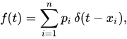
This substantially unifies the treatment of discrete and continuous probability distributions. The above expression allows for determining statistical characteristics of such a discrete variable (such as the mean, variance, and kurtosis), starting from the formulas given for a continuous distribution of the probability.

Families of densities

It is common for probability density functions (and probability mass functions) to be parametrized—that is, to be characterized by unspecified parameters. For example, the normal distribution is parametrized in terms of the mean and the variance, denoted by ${\displaystyle \mu }$ and ${\displaystyle {\sigma }^2}$ respectively, giving the family of densities $${\displaystyle f(x;\mu ,{\sigma }^2)=\frac{1}{\sigma \sqrt{2\pi }}{e}^{-\frac{1}{2}{\left(\frac{x-\mu }{\sigma }\right)}^2}.}$$ Different values of the parameters describe different distributions of different random variables on the same sample space (the same set of all possible values of the variable); this sample space is the domain of the family of random variables that this family of distributions describes. A given set of parameters describes a single distribution within the family sharing the functional form of the density. From the perspective of a given distribution, the parameters are constants, and terms in a density function that contain only parameters, but not variables, are part of the normalization factor of a distribution (the multiplicative factor that ensures that the area under the density—the probability of something in the domain occurring— equals 1). This normalization factor is outside the kernel of the distribution.

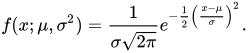
Since the parameters are constants, reparametrizing a density in terms of different parameters to give a characterization of a different random variable in the family, means simply substituting the new parameter values into the formula in place of the old ones.

Densities associated with multiple variables

For continuous random variables X₁, ..., X_n, it is also possible to define a probability density function associated to the set as a whole, often called joint probability density function. This density function is defined as a function of the n variables, such that, for any domain D in the n-dimensional space of the values of the variables X₁, ..., X_n, the probability that a realisation of the set variables falls inside the domain D is $${\displaystyle Pr\left(X_1,\dots ,X_n\in D\right)={\int }_D{f}_{X_1,\dots ,X_n}(x_1,\dots ,x_n)d{x}_1\cdots d{x}_n.}$$

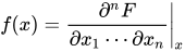
If F(x₁, ..., x_n) = Pr(X₁ ≤ x₁, ..., X_n ≤ x_n) is the cumulative distribution function of the vector (X₁, ..., X_n), then the joint probability density function can be computed as a partial derivative $${\displaystyle f(x)={\frac{{\mathrm{\partial }}^{n}F}{\mathrm{\partial }{x}_1\cdots \mathrm{\partial }{x}_n}|}_x}$$

Marginal densities

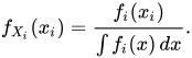
For i = 1, 2, ..., n, let f_Xi(x_i) be the probability density function associated with variable X_i alone. This is called the marginal density function, and can be deduced from the probability density associated with the random variables X₁, ..., X_n by integrating over all values of the other n − 1 variables: $${\displaystyle f_{X_i}(x_i)=\int f(x_1,\dots ,x_n)d{x}_1\cdots d{x}_{i-1}d{x}_{i+1}\cdots d{x}_n.}$$

Independence

Continuous random variables X₁, ..., X_n admitting a joint density are all independent from each other if $${\displaystyle f_{X_1,\dots ,X_n}(x_1,\dots ,x_n)=f_{X_1}(x_1)\cdots f_{X_n}(x_n).}$$

Corollary

If the joint probability density function of a vector of n random variables can be factored into a product of n functions of one variable $${\displaystyle f_{X_1,\dots ,X_n}(x_1,\dots ,x_n)=f_1(x_1)\cdots f_n(x_n),}$$ (where each f_i is not necessarily a density) then the n variables in the set are all independent from each other, and the marginal probability density function of each of them is given by $${\displaystyle f_{X_i}(x_i)=\frac{f_i(x_i)}{\int f_i(x)dx}.}$$

Example

This elementary example illustrates the above definition of multidimensional probability density functions in the simple case of a function of a set of two variables. Let us call ${\displaystyle \overrightarrow{R}}$ a 2-dimensional random vector of coordinates (X, Y): the probability to obtain ${\displaystyle \overrightarrow{R}}$ in the quarter plane of positive x and y is $${\displaystyle Pr\left(X>0,Y>0\right)={\int }_0^{\mathrm{\infty }}{\int }_0^{\mathrm{\infty }}{f}_{X,Y}(x,y)dxdy.}$$

Function of random variables and change of variables in the probability density function

If the probability density function of a random variable (or vector) X is given as f_X(x), it is possible (but often not necessary; see below) to calculate the probability density function of some variable Y = g(X). This is also called a "change of variable" and is in practice used to generate a random variable of arbitrary shape f_g(X) = f_Y using a known (for instance, uniform) random number generator.

It is tempting to think that in order to find the expected value E(g(X)), one must first find the probability density f_g(X) of the new random variable Y = g(X). However, rather than computing $${\displaystyle \mathrm{E}(g(X))={\int }_{-\mathrm{\infty }}^{\mathrm{\infty }}y{f}_{g(X)}(y)dy,}$$ one may find instead $${\displaystyle \mathrm{E}(g(X))={\int }_{-\mathrm{\infty }}^{\mathrm{\infty }}g(x)f_X(x)dx.}$$

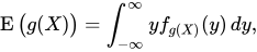
The values of the two integrals are the same in all cases in which both X and g(X) actually have probability density functions. It is not necessary that g be a one-to-one function. In some cases the latter integral is computed much more easily than the former. See Law of the unconscious statistician.

Scalar to scalar

Let ${\displaystyle g:\mathbb{R}\to \mathbb{R}}$ be a monotonic function, then the resulting density function is $${\displaystyle f_Y(y)=f_X(g^{-1}(y))\left|\frac{d}{dy}(g^{-1}(y))\right|.}$$

Here g⁻¹ denotes the inverse function.

This follows from the fact that the probability contained in a differential area must be invariant under change of variables. That is, $${\displaystyle \left|f_Y(y)dy\right|=\left|f_X(x)dx\right|,}$$ or $${\displaystyle f_Y(y)=\left|\frac{dx}{dy}\right|f_X(x)=\left|\frac{d}{dy}(x)\right|f_X(x)=\left|\frac{d}{dy}(g^{-1}(y))\right|f_X(g^{-1}(y))=\left|{\left(g^{-1}\right)}^{\prime }(y)\right|\cdot f_X(g^{-1}(y)).}$$

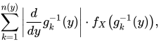
For functions that are not monotonic, the probability density function for y is $${\displaystyle \sum _{k=1}^{n(y)}\left|\frac{d}{dy}{g}_k^{-1}(y)\right|\cdot f_X(g_k^{-1}(y)),}$$ where n(y) is the number of solutions in x for the equation ${\displaystyle g(x)=y}$, and ${\displaystyle g_k^{-1}(y)}$ are these solutions.

Vector to vector

Suppose x is an n-dimensional random variable with joint density f. If y = G(x), where G is a bijective, differentiable function, then y has density p_Y: $${\displaystyle p_Y(\mathbf{y})=f(G^{-1}(\mathbf{y}))\left|det\left[{\frac{d{G}^{-1}(\mathbf{z})}{d\mathbf{z}}|}_{\mathbf{z}=\mathbf{y}}\right]\right|}$$ with the differential regarded as the Jacobian of the inverse of G(⋅), evaluated at y.

For example, in the 2-dimensional case x = (x₁, x₂), suppose the transform G is given as y₁ = G₁(x₁, x₂), y₂ = G₂(x₁, x₂) with inverses x₁ = G₁⁻¹(y₁, y₂), x₂ = G₂⁻¹(y₁, y₂). The joint distribution for y = (y₁, y₂) has density $${\displaystyle p_{Y_1,Y_2}(y_1,y_2)=f_{X_1,X_2}(G_1^{-1}(y_1,y_2),G_2^{-1}(y_1,y_2))\left|\frac{\mathrm{\partial }{G}_1^{-1}}{\mathrm{\partial }{y}_1}\frac{\mathrm{\partial }{G}_2^{-1}}{\mathrm{\partial }{y}_2}-\frac{\mathrm{\partial }{G}_1^{-1}}{\mathrm{\partial }{y}_2}\frac{\mathrm{\partial }{G}_2^{-1}}{\mathrm{\partial }{y}_1}\right|.}$$

Vector to scalar

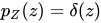
Let ${\displaystyle V:{\mathbb{R}}^n\to \mathbb{R}}$ be a differentiable function and ${\displaystyle X}$ be a random vector taking values in ${\displaystyle {\mathbb{R}}^n}$, ${\displaystyle f_X}$ be the probability density function of ${\displaystyle X}$ and ${\displaystyle \delta (\cdot )}$ be the Dirac delta function. It is possible to use the formulas above to determine ${\displaystyle f_Y}$, the probability density function of ${\displaystyle Y=V(X)}$, which will be given by $${\displaystyle f_Y(y)={\int }_{{\mathbb{R}}^n}{f}_X(\mathbf{x})\delta (y-V(\mathbf{x}))d\mathbf{x}.}$$

This result leads to the law of the unconscious statistician: $${\displaystyle \begin{array}{rl}{\mathrm{E}}_Y[Y]& ={\int }_{\mathbb{R}}y{f}_Y(y)dy\\ & ={\int }_{\mathbb{R}}y{\int }_{{\mathbb{R}}^n}{f}_X(\mathbf{x})\delta (y-V(\mathbf{x}))d\mathbf{x}dy\\ & ={\int }_{{\mathbb{R}}^n}{\int }_{\mathbb{R}}y{f}_X(\mathbf{x})\delta (y-V(\mathbf{x}))dyd\mathbf{x}\\ & ={\int }_{{\mathbb{R}}^n}V(\mathbf{x})f_X(\mathbf{x})d\mathbf{x}={\mathrm{E}}_X[V(X)].\end{array}}$$

Proof:

Let ${\displaystyle Z}$ be a collapsed random variable with probability density function ${\displaystyle p_Z(z)=\delta (z)}$ (i.e., a constant equal to zero). Let the random vector ${\displaystyle \tilde{X}}$ and the transform ${\displaystyle H}$ be defined as $${\displaystyle H(Z,X)=\left[\begin{array}{c}Z+V(X)\\ X\end{array}\right]=\left[\begin{array}{c}Y\\ \tilde{X}\end{array}\right].}$$

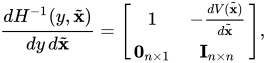
It is clear that ${\displaystyle H}$ is a bijective mapping, and the Jacobian of ${\displaystyle H^{-1}}$ is given by: $${\displaystyle \frac{d{H}^{-1}(y,\tilde{\mathbf{x}})}{dyd\tilde{\mathbf{x}}}=\left[\begin{array}{cc}1& -\frac{dV(\tilde{\mathbf{x}})}{d\tilde{\mathbf{x}}}\\ {\mathbf{0}}_{n\times 1}& {\mathbf{I}}_{n\times n}\end{array}\right],}$$ which is an upper triangular matrix with ones on the main diagonal, therefore its determinant is 1. Applying the change of variable theorem from the previous section we obtain that $${\displaystyle f_{Y,X}(y,x)=f_X(\mathbf{x})\delta (y-V(\mathbf{x})),}$$ which if marginalized over ${\displaystyle x}$ leads to the desired probability density function.

Sums of independent random variables

See also: List of convolutions of probability distributions

The probability density function of the sum of two independent random variables U and V, each of which has a probability density function, is the convolution of their separate density functions: $${\displaystyle f_{U+V}(x)={\int }_{-\mathrm{\infty }}^{\mathrm{\infty }}{f}_U(y)f_V(x-y)dy=\left(f_U\ast f_V\right)(x)}$$

It is possible to generalize the previous relation to a sum of N independent random variables, with densities U₁, ..., U_N: $${\displaystyle f_{U_1+\cdots +U}(x)=\left(f_{U_1}\ast \cdots \ast f_{U_N}\right)(x)}$$

This can be derived from a two-way change of variables involving Y = U + V and Z = V, similarly to the example below for the quotient of independent random variables.

Products and quotients of independent random variables

See also: Product distribution and Ratio distribution

Given two independent random variables U and V, each of which has a probability density function, the density of the product Y = UV and quotient Y = U/V can be computed by a change of variables.

Example: Quotient distribution

To compute the quotient Y = U/V of two independent random variables U and V, define the following transformation: $${\displaystyle \begin{array}{rl}Y& =U/V\\ Z& =V\end{array}}$$

Then, the joint density p(y,z) can be computed by a change of variables from U,V to Y,Z, and Y can be derived by marginalizing out Z from the joint density.

The inverse transformation is $${\displaystyle \begin{array}{rl}U& =YZ\\ V& =Z\end{array}}$$

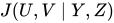
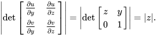
The absolute value of the Jacobian matrix determinant ${\displaystyle J(U,V\mid Y,Z)}$ of this transformation is: $${\displaystyle \left|det\left[\begin{array}{cc}\frac{\mathrm{\partial }u}{\mathrm{\partial }y}& \frac{\mathrm{\partial }u}{\mathrm{\partial }z}\\ \frac{\mathrm{\partial }v}{\mathrm{\partial }y}& \frac{\mathrm{\partial }v}{\mathrm{\partial }z}\end{array}\right]\right|=\left|det\left[\begin{array}{cc}z& y\\ 0& 1\end{array}\right]\right|=|z|.}$$

Thus: $${\displaystyle p(y,z)=p(u,v)J(u,v\mid y,z)=p(u)p(v)J(u,v\mid y,z)=p_U(yz)p_V(z)|z|.}$$

And the distribution of Y can be computed by marginalizing out Z: $${\displaystyle p(y)={\int }_{-\mathrm{\infty }}^{\mathrm{\infty }}{p}_U(yz)p_V(z)|z|dz}$$

This method crucially requires that the transformation from U,V to Y,Z be bijective. The above transformation meets this because Z can be mapped directly back to V, and for a given V the quotient U/V is monotonic. This is similarly the case for the sum U + V, difference U − V and product UV.

Exactly the same method can be used to compute the distribution of other functions of multiple independent random variables.

Example: Quotient of two standard normals

Given two standard normal variables U and V, the quotient can be computed as follows. First, the variables have the following density functions: $${\displaystyle \begin{array}{rl}p(u)& =\frac{1}{\sqrt{2\pi }}{e}^{-u^2/2}\\ p(v)& =\frac{1}{\sqrt{2\pi }}{e}^{-v^2/2}\end{array}}$$

We transform as described above: $${\displaystyle \begin{array}{rl}Y& =U/V\\ Z& =V\end{array}}$$

This leads to: $${\displaystyle \begin{array}{rl}p(y)& ={\int }_{-\mathrm{\infty }}^{\mathrm{\infty }}{p}_U(yz)p_V(z)|z|dz\\ & ={\int }_{-\mathrm{\infty }}^{\mathrm{\infty }}\frac{1}{\sqrt{2\pi }}{e}^{-\frac{1}{2}{y}^2{z}^2}\frac{1}{\sqrt{2\pi }}{e}^{-\frac{1}{2}{z}^2}|z|dz\\ & ={\int }_{-\mathrm{\infty }}^{\mathrm{\infty }}\frac{1}{2\pi }{e}^{-\frac{1}{2}\left(y^2+1\right)z^2}|z|dz\\ & =2{\int }_0^{\mathrm{\infty }}\frac{1}{2\pi }{e}^{-\frac{1}{2}\left(y^2+1\right)z^2}zdz\\ & ={\int }_0^{\mathrm{\infty }}\frac{1}{\pi }{e}^{-\left(y^2+1\right)u}du& & u=\frac{1}{2}{z}^2\\ & ={-\frac{1}{\pi \left(y^2+1\right)}{e}^{-\left(y^2+1\right)u}|}_{u=0}^{\mathrm{\infty }}\\ & =\frac{1}{\pi \left(y^2+1\right)}\end{array}}$$

This is the density of a standard Cauchy distribution.

Scattering

From Wikipedia, the free encyclopedia
https://en.wikipedia.org/wiki/Scattering

 

Scattering
Feynman diagram of scattering between two electrons by emission of a virtual photon

A wine glass in an LCD projector's light beam makes the beam scatter.

In physics, scattering is a wide range of physical processes where moving particles or radiation of some form, such as light or sound, are forced to deflect from a straight trajectory or are blocked by localized non-uniformities (including particles, matter, interfaces, and radiation) in the propagation medium through which they pass. In conventional use, this also includes deviation of reflected radiation from the angle predicted by the law of reflection. Reflections of radiation that undergo scattering are often called diffuse reflections and unscattered reflections are called specular (mirror-like) reflections.

Originally, the term was confined to light scattering (going back at least as far as Isaac Newton in the 17th century). As more "ray"-like phenomena were discovered, the idea of scattering was extended to them, so that William Herschel could refer to the scattering of "heat rays" (not then recognized as electromagnetic in nature) in 1800. John Tyndall, a pioneer in light scattering research, noted the connection between light scattering and acoustic scattering in the 1870s. Near the end of the 19th century, the scattering of cathode rays (electron beams) and X-rays was observed and discussed. With the discovery of subatomic particles (e.g. Ernest Rutherford in 1911) and the development of quantum theory in the 20th century, the sense of the term became broader as it was recognized that the same mathematical frameworks used in light scattering could be applied to many other phenomena.

Scattering can refer to the consequences of particle-particle collisions between molecules, atoms, electrons, photons and other particles. Examples include: cosmic ray scattering in the Earth's upper atmosphere; particle collisions inside particle accelerators; electron scattering by gas atoms in fluorescent lamps; and neutron scattering inside nuclear reactors.^[7]

The types of non-uniformities which can cause scattering, sometimes known as scatterers or scattering centers, are too numerous to list, but a small sample includes particles, bubbles, droplets, density fluctuations in fluids, crystallites in polycrystalline solids, defects in monocrystalline solids, surface roughness, cells in organisms, and textile fibers in clothing. The effects of such features on the path of almost any type of propagating wave or moving particle can be described in the framework of scattering theory.

Some areas where scattering and scattering theory are significant include radar sensing, medical ultrasound, semiconductor wafer inspection, polymerization process monitoring, acoustic tiling, free-space communications and computer-generated imagery. Particle-particle scattering theory is important in areas such as particle physics, atomic, molecular, and optical physics, nuclear physics and astrophysics. In particle physics the quantum interaction and scattering of fundamental particles is described by the Scattering Matrix or S-Matrix, introduced and developed by John Archibald Wheeler and Werner Heisenberg.

Scattering is quantified using many different concepts, including scattering cross section (σ), attenuation coefficients, the bidirectional scattering distribution function (BSDF), S-matrices, and mean free path.

Single and multiple scattering

Zodiacal light is a faint, diffuse glow visible in the night sky. The phenomenon stems from the scattering of sunlight by interplanetary dust spread throughout the plane of the Solar System.

When radiation is only scattered by one localized scattering center, this is called single scattering. It is more common that scattering centers are grouped together; in such cases, radiation may scatter many times, in what is known as multiple scattering. The main difference between the effects of single and multiple scattering is that single scattering can usually be treated as a random phenomenon, whereas multiple scattering, somewhat counterintuitively, can be modeled as a more deterministic process because the combined results of a large number of scattering events tend to average out. Multiple scattering can thus often be modeled well with diffusion theory.

Because the location of a single scattering center is not usually well known relative to the path of the radiation, the outcome, which tends to depend strongly on the exact incoming trajectory, appears random to an observer. This type of scattering would be exemplified by an electron being fired at an atomic nucleus. In this case, the atom's exact position relative to the path of the electron is unknown and would be unmeasurable, so the exact trajectory of the electron after the collision cannot be predicted. Single scattering is therefore often described by probability distributions.

With multiple scattering, the randomness of the interaction tends to be averaged out by a large number of scattering events, so that the final path of the radiation appears to be a deterministic distribution of intensity. This is exemplified by a light beam passing through thick fog. Multiple scattering is highly analogous to diffusion, and the terms multiple scattering and diffusion are interchangeable in many contexts. Optical elements designed to produce multiple scattering are thus known as diffusers. Coherent backscattering, an enhancement of backscattering that occurs when coherent radiation is multiply scattered by a random medium, is usually attributed to weak localization.

Not all single scattering is random, however. A well-controlled laser beam can be exactly positioned to scatter off a microscopic particle with a deterministic outcome, for instance. Such situations are encountered in radar scattering as well, where the targets tend to be macroscopic objects such as people or aircraft.

Similarly, multiple scattering can sometimes have somewhat random outcomes, particularly with coherent radiation. The random fluctuations in the multiply scattered intensity of coherent radiation are called speckles. Speckle also occurs if multiple parts of a coherent wave scatter from different centers. In certain rare circumstances, multiple scattering may only involve a small number of interactions such that the randomness is not completely averaged out. These systems are considered to be some of the most difficult to model accurately.

The description of scattering and the distinction between single and multiple scattering are tightly related to wave–particle duality.

Theory

Scattering theory is a framework for studying and understanding the scattering of waves and particles. Wave scattering corresponds to the collision and scattering of a wave with some material object, for instance sunlight scattered by rain drops to form a rainbow. Scattering also includes the interaction of billiard balls on a table, the Rutherford scattering (or angle change) of alpha particles by gold nuclei, the Bragg scattering (or diffraction) of electrons and X-rays by a cluster of atoms, and the inelastic scattering of a fission fragment as it traverses a thin foil. More precisely, scattering consists of the study of how solutions of partial differential equations, propagating freely "in the distant past", come together and interact with one another or with a boundary condition, and then propagate away "to the distant future".

The direct scattering problem is the problem of determining the distribution of scattered radiation/particle flux basing on the characteristics of the scatterer. The inverse scattering problem is the problem of determining the characteristics of an object (e.g., its shape, internal constitution) from measurement data of radiation or particles scattered from the object.

Attenuation due to scattering

Equivalent quantities used in the theory of scattering from composite specimens, but with a variety of units

When the target is a set of many scattering centers whose relative position varies unpredictably, it is customary to think of a range equation whose arguments take different forms in different application areas. In the simplest case consider an interaction that removes particles from the "unscattered beam" at a uniform rate that is proportional to the incident number of particles per unit area per unit time (${\displaystyle I}$), i.e. that

$${\displaystyle \frac{dI}{dx}=-QI}$$

where Q is an interaction coefficient and x is the distance traveled in the target.

The above ordinary first-order differential equation has solutions of the form:

$${\displaystyle I=I_o{e}^{-Q\mathrm{\Delta }x}=I_o{e}^{-\frac{\mathrm{\Delta }x}{\lambda }}=I_o{e}^{-\sigma (\eta \mathrm{\Delta }x)}=I_o{e}^{-\frac{\rho \mathrm{\Delta }x}{\tau }},}$$

where I_o is the initial flux, path length Δx ≡ x − x_o, the second equality defines an interaction mean free path λ, the third uses the number of targets per unit volume η to define an area cross-section σ, and the last uses the target mass density ρ to define a density mean free path τ. Hence one converts between these quantities via Q = 1/λ = ησ = ρ/τ, as shown in the figure at left.

In electromagnetic absorption spectroscopy, for example, interaction coefficient (e.g. Q in cm⁻¹) is variously called opacity, absorption coefficient, and attenuation coefficient. In nuclear physics, area cross-sections (e.g. σ in barns or units of 10⁻²⁴ cm²), density mean free path (e.g. τ in grams/cm²), and its reciprocal the mass attenuation coefficient (e.g. in cm²/gram) or area per nucleon are all popular, while in electron microscopy the inelastic mean free path (e.g. λ in nanometers) is often discussed instead.

Elastic and inelastic scattering

The term "elastic scattering" implies that the internal states of the scattering particles do not change, and hence they emerge unchanged from the scattering process. In inelastic scattering, by contrast, the particles' internal state is changed, which may amount to exciting some of the electrons of a scattering atom, or the complete annihilation of a scattering particle and the creation of entirely new particles.

The example of scattering in quantum chemistry is particularly instructive, as the theory is reasonably complex while still having a good foundation on which to build an intuitive understanding. When two atoms are scattered off one another, one can understand them as being the bound state solutions of some differential equation. Thus, for example, the hydrogen atom corresponds to a solution to the Schrödinger equation with a negative inverse-power (i.e., attractive Coulombic) central potential. The scattering of two hydrogen atoms will disturb the state of each atom, resulting in one or both becoming excited, or even ionized, representing an inelastic scattering process.

The term "deep inelastic scattering" refers to a special kind of scattering experiment in particle physics.

Mathematical framework

In mathematics, scattering theory deals with a more abstract formulation of the same set of concepts. For example, if a differential equation is known to have some simple, localized solutions, and the solutions are a function of a single parameter, that parameter can take the conceptual role of time. One then asks what might happen if two such solutions are set up far away from each other, in the "distant past", and are made to move towards each other, interact (under the constraint of the differential equation) and then move apart in the "future". The scattering matrix then pairs solutions in the "distant past" to those in the "distant future".

Solutions to differential equations are often posed on manifolds. Frequently, the means to the solution requires the study of the spectrum of an operator on the manifold. As a result, the solutions often have a spectrum that can be identified with a Hilbert space, and scattering is described by a certain map, the S matrix, on Hilbert spaces. Solutions with a discrete spectrum correspond to bound states in quantum mechanics, while a continuous spectrum is associated with scattering states. The study of inelastic scattering then asks how discrete and continuous spectra are mixed together.

An important, notable development is the inverse scattering transform, central to the solution of many exactly solvable models.

Theoretical physics

Top: the real part of a plane wave travelling upwards. Bottom: The real part of the field after inserting in the path of the plane wave a small transparent disk of index of refraction higher than the index of the surrounding medium. This object scatters part of the wave field, although at any individual point, the wave's frequency and wavelength remain intact.

In mathematical physics, scattering theory is a framework for studying and understanding the interaction or scattering of solutions to partial differential equations. In acoustics, the differential equation is the wave equation, and scattering studies how its solutions, the sound waves, scatter from solid objects or propagate through non-uniform media (such as sound waves, in sea water, coming from a submarine). In the case of classical electrodynamics, the differential equation is again the wave equation, and the scattering of light or radio waves is studied. In particle physics, the equations are those of Quantum electrodynamics, Quantum chromodynamics and the Standard Model, the solutions of which correspond to fundamental particles.

In regular quantum mechanics, which includes quantum chemistry, the relevant equation is the Schrödinger equation, although equivalent formulations, such as the Lippmann-Schwinger equation and the Faddeev equations, are also largely used. The solutions of interest describe the long-term motion of free atoms, molecules, photons, electrons, and protons. The scenario is that several particles come together from an infinite distance away. These reagents then collide, optionally reacting, getting destroyed or creating new particles. The products and unused reagents then fly away to infinity again. (The atoms and molecules are effectively particles for our purposes. Also, under everyday circumstances, only photons are being created and destroyed.) The solutions reveal which directions the products are most likely to fly off to and how quickly. They also reveal the probability of various reactions, creations, and decays occurring. There are two predominant techniques of finding solutions to scattering problems: partial wave analysis, and the Born approximation.

Electromagnetics

A Feynman diagram of scattering between two electrons by emission of a virtual photon

Electromagnetic waves are one of the best known and most commonly encountered forms of radiation that undergo scattering. Scattering of light and radio waves (especially in radar) is particularly important. Several different aspects of electromagnetic scattering are distinct enough to have conventional names. Major forms of elastic light scattering (involving negligible energy transfer) are Rayleigh scattering and Mie scattering. Inelastic scattering includes Brillouin scattering, Raman scattering, inelastic X-ray scattering and Compton scattering.

Light scattering is one of the two major physical processes that contribute to the visible appearance of most objects, the other being absorption. Surfaces described as white owe their appearance to multiple scattering of light by internal or surface inhomogeneities in the object, for example by the boundaries of transparent microscopic crystals that make up a stone or by the microscopic fibers in a sheet of paper. More generally, the gloss (or lustre or sheen) of the surface is determined by scattering. Highly scattering surfaces are described as being dull or having a matte finish, while the absence of surface scattering leads to a glossy appearance, as with polished metal or stone.

Spectral absorption, the selective absorption of certain colors, determines the color of most objects with some modification by elastic scattering. The apparent blue color of veins in skin is a common example where both spectral absorption and scattering play important and complex roles in the coloration. Light scattering can also create color without absorption, often shades of blue, as with the sky (Rayleigh scattering), the human blue iris, and the feathers of some birds (Prum et al. 1998). However, resonant light scattering in nanoparticles can produce many different highly saturated and vibrant hues, especially when surface plasmon resonance is involved (Roqué et al. 2006).

Models of light scattering can be divided into three domains based on a dimensionless size parameter, α which is defined as: $${\displaystyle \alpha =\pi D_{\text{p}}/\lambda ,}$$ where πD_p is the circumference of a particle and λ is the wavelength of incident radiation in the medium. Based on the value of α, these domains are:

• α ≪ 1: Rayleigh scattering (small particle compared to wavelength of light);
• α ≈ 1: Mie scattering (particle about the same size as wavelength of light, valid only for spheres);
• α ≫ 1: geometric scattering (particle much larger than wavelength of light).

Rayleigh scattering is a process in which electromagnetic radiation (including light) is scattered by a small spherical volume of variant refractive indexes, such as a particle, bubble, droplet, or even a density fluctuation. This effect was first modeled successfully by Lord Rayleigh, from whom it gets its name. In order for Rayleigh's model to apply, the sphere must be much smaller in diameter than the wavelength (λ) of the scattered wave; typically the upper limit is taken to be about 1/10 the wavelength. In this size regime, the exact shape of the scattering center is usually not very significant and can often be treated as a sphere of equivalent volume. The inherent scattering that radiation undergoes passing through a pure gas is due to microscopic density fluctuations as the gas molecules move around, which are normally small enough in scale for Rayleigh's model to apply. This scattering mechanism is the primary cause of the blue color of the Earth's sky on a clear day, as the shorter blue wavelengths of sunlight passing overhead are more strongly scattered than the longer red wavelengths according to Rayleigh's famous 1/λ⁴ relation. Along with absorption, such scattering is a major cause of the attenuation of radiation by the atmosphere. The degree of scattering varies as a function of the ratio of the particle diameter to the wavelength of the radiation, along with many other factors including polarization, angle, and coherence.

For larger diameters, the problem of electromagnetic scattering by spheres was first solved by Gustav Mie, and scattering by spheres larger than the Rayleigh range is therefore usually known as Mie scattering. In the Mie regime, the shape of the scattering center becomes much more significant and the theory only applies well to spheres and, with some modification, spheroids and ellipsoids. Closed-form solutions for scattering by certain other simple shapes exist, but no general closed-form solution is known for arbitrary shapes.

Both Mie and Rayleigh scattering are considered elastic scattering processes, in which the energy (and thus wavelength and frequency) of the light is not substantially changed. However, electromagnetic radiation scattered by moving scattering centers does undergo a Doppler shift, which can be detected and used to measure the velocity of the scattering center/s in forms of techniques such as lidar and radar. This shift involves a slight change in energy.

At values of the ratio of particle diameter to wavelength more than about 10, the laws of geometric optics are mostly sufficient to describe the interaction of light with the particle. Mie theory can still be used for these larger spheres, but the solution often becomes numerically unwieldy.

For modeling of scattering in cases where the Rayleigh and Mie models do not apply such as larger, irregularly shaped particles, there are many numerical methods that can be used. The most common are finite-element methods which solve Maxwell's equations to find the distribution of the scattered electromagnetic field. Sophisticated software packages exist which allow the user to specify the refractive index or indices of the scattering feature in space, creating a 2- or sometimes 3-dimensional model of the structure. For relatively large and complex structures, these models usually require substantial execution times on a computer.

Electrophoresis involves the migration of macromolecules under the influence of an electric field. Electrophoretic light scattering involves passing an electric field through a liquid which makes particles move. The bigger the charge is on the particles, the faster they are able to move.