Eigenvalues and eigenvectors

From Wikipedia, the free encyclopedia

https://en.wikipedia.org/wiki/Eigenvalues_and_eigenvectors

In linear algebra, an eigenvector (/ˈaɪɡən-/ EYE-gən-) or characteristic vector is a (nonzero) vector that has its direction unchanged (or reversed) by a given linear transformation. More precisely, an eigenvector ${\displaystyle \mathbf{v}}$ of a linear transformation ${\displaystyle T}$ is scaled by a constant factor ${\displaystyle \lambda }$ when the linear transformation is applied to it: ⁠${\displaystyle T\mathbf{v}=\lambda \mathbf{v}}$⁠. The corresponding eigenvalue, characteristic value, or characteristic root is the multiplying factor ${\displaystyle \lambda }$ (possibly a negative or complex number).

Geometrically, vectors are multi-dimensional quantities with magnitude and direction, often pictured as arrows. A linear transformation rotates, stretches, or shears the vectors upon which it acts. A linear transformation's eigenvectors are those vectors that are only stretched or shrunk, with neither rotation nor shear. The corresponding eigenvalue is the factor by which an eigenvector is stretched or shrunk. If the eigenvalue is negative, then the eigenvector's direction is reversed.

The eigenvectors and eigenvalues of a linear transformation serve to characterize it, and so they play important roles in all areas where linear algebra is applied, from geology to quantum mechanics. In particular, it is often the case that a system is represented by a linear transformation whose outputs are fed as inputs to the same transformation (feedback). In such an application, the largest eigenvalue is of particular importance, because it governs the long-term behavior of the system after many applications of the linear transformation, and the associated eigenvector is the steady state of the system.

Matrices

For an ${\displaystyle n\times n}$ matrix ⁠${\displaystyle A}$⁠ and a nonzero ⁠${\displaystyle n}$⁠-vector ⁠${\displaystyle \mathbf{v}}$⁠, if multiplying ⁠${\displaystyle A}$⁠ by ${\displaystyle \mathbf{v}}$ (denoted ⁠${\displaystyle A\mathbf{v}}$⁠) simply scales ${\displaystyle \mathbf{v}}$ by a factor ⁠${\displaystyle \lambda }$⁠, where ⁠${\displaystyle \lambda }$⁠ is a scalar, then ${\displaystyle \mathbf{v}}$ is called an eigenvector of ⁠${\displaystyle A}$⁠, and ⁠${\displaystyle \lambda }$⁠ is the corresponding eigenvalue. This relationship can be expressed as: ⁠${\displaystyle A\mathbf{v}=\lambda \mathbf{v}}$⁠.

Given an ⁠${\displaystyle n}$⁠-dimensional vector space and a choice of basis, there is a direct correspondence between linear transformations from the vector space into itself and ⁠${\displaystyle n\times n}$⁠ square matrices. Hence, in a finite-dimensional vector space, it is equivalent to define eigenvalues and eigenvectors using either the language of linear transformations, or the language of matrices.

Overview

Eigenvalues and eigenvectors feature prominently in the analysis of linear transformations. The prefix eigen- is adopted from the German eigen (cognate with the English word own) for 'proper', 'characteristic', 'own'. Originally used to study principal axes of the rotational motion of rigid bodies, eigenvalues and eigenvectors have a wide range of applications, for example in stability analysis, vibration analysis, atomic orbitals, facial recognition, and matrix diagonalization.

In essence, an eigenvector v of a linear transformation T is a nonzero vector that, when T is applied to it, does not change direction. Applying T to the eigenvector only scales the eigenvector by the scalar value λ, called an eigenvalue. This condition can be written as the equation $${\displaystyle T(\mathbf{v})=\lambda \mathbf{v},}$$ referred to as the eigenvalue equation or eigenequation. In general, λ may be any scalar. For example, λ may be negative, in which case the eigenvector reverses direction as part of the scaling, or it may be zero, or complex.

In this shear mapping, the red arrow changes direction but the blue arrow does not. The blue arrow is an eigenvector of this shear mapping because it does not change direction, and since its length is unchanged, its eigenvalue is 1.

A 2 × 2 real and symmetric matrix representing a stretching and shearing of the plane. The eigenvectors of the matrix (red lines) are the two special directions such that every point on them will just slide on them.

The example here, based on the Mona Lisa, provides a simple illustration. Each point on the painting can be represented as a vector pointing from the center of the painting to that point. The linear transformation in this example is called a shear mapping. Points in the top half are moved to the right, and points in the bottom half are moved to the left, proportional to how far they are from the horizontal axis that goes through the middle of the painting. The vectors pointing to each point in the original image are therefore tilted right or left, and made longer or shorter by the transformation. Points along the horizontal axis do not move at all when this transformation is applied. Therefore, any vector that points directly to the right or left with no vertical component is an eigenvector of this transformation, because the mapping does not change its direction. Moreover, these eigenvectors all have an eigenvalue equal to one, because the mapping does not change their length either.

Animated examples of eigenvectors and real eigenvalues for several non-symmetric 2D linear transformations

Linear transformations can take many different forms, mapping vectors in a variety of vector spaces, so the eigenvectors can also take many forms. For example, the linear transformation could be a differential operator like ⁠${\displaystyle \frac{d}{dx}}$⁠, in which case the eigenvectors are functions called eigenfunctions that are scaled by that differential operator, such as $${\displaystyle \frac{d}{dx}{e}^{\lambda x}=\lambda e^{\lambda x}.}$$ Alternatively, the linear transformation could take the form of an n × n matrix, in which case the eigenvectors are n × 1 matrices.

If the linear transformation is expressed in the form of an n × n matrix A, then the eigenvalue equation for a linear transformation above can be rewritten as the matrix multiplication $${\displaystyle A\mathbf{v}=\lambda \mathbf{v},}$$ where the eigenvector v is an n × 1 matrix. For a matrix, eigenvalues and eigenvectors can be used to decompose the matrix; for example, by diagonalizing it. Eigenvalues and eigenvectors give rise to many closely related mathematical concepts, and the prefix eigen- is applied liberally when naming them:

• The set of all eigenvectors of a linear transformation, each paired with its corresponding eigenvalue, is called the eigensystem of that transformation.
• The set of all eigenvectors of T corresponding to the same eigenvalue, together with the zero vector, is called an eigenspace, or the characteristic space of T associated with that eigenvalue.
• If a set of eigenvectors of T forms a basis of the domain of T, then this basis is called an eigenbasis.

Additional animations of eigenvectors and eigenvalues in two dimensions, including symmetric transformations and transformations with complex eigenvalues, are available at Wikimedia Commons.

History

Eigenvalues are often introduced in the context of linear algebra or matrix theory. Historically, however, they arose in the study of quadratic forms and differential equations.

In the 18th century, Leonhard Euler studied the rotational motion of a rigid body, and discovered the importance of the principal axes. Joseph-Louis Lagrange realized that the principal axes are the eigenvectors of the inertia matrix.

In the early 19th century, Augustin-Louis Cauchy saw how their work could be used to classify the quadric surfaces, and generalized it to arbitrary dimensions. Cauchy also coined the term racine caractéristique (characteristic root), for what is now called eigenvalue; his term survives in characteristic equation.

Later, Joseph Fourier used the work of Lagrange and Pierre-Simon Laplace to solve the heat equation by separation of variables in his 1822 treatise The Analytic Theory of Heat (Théorie analytique de la chaleur). Charles-François Sturm elaborated on Fourier's ideas further, and brought them to the attention of Cauchy, who combined them with his own ideas and arrived at the fact that real symmetric matrices have real eigenvalues. This was extended by Charles Hermite in 1855 to what are now called Hermitian matrices.

Around the same time, Francesco Brioschi proved that the eigenvalues of orthogonal matrices lie on the unit circle, and Alfred Clebsch found the corresponding result for skew-symmetric matrices. Finally, Karl Weierstrass clarified an important aspect in the stability theory started by Laplace, by realizing that defective matrices can cause instability.

In the meantime, Joseph Liouville studied eigenvalue problems similar to those of Sturm; the discipline that grew out of their work is now called Sturm–Liouville theory. Schwarz studied the first eigenvalue of Laplace's equation on general domains towards the end of the 19th century, while Poincaré studied Poisson's equation a few years later.

At the start of the 20th century, David Hilbert studied the eigenvalues of integral operators by viewing the operators as infinite matrices. He was the first to use the German word eigen, which means "own", to denote eigenvalues and eigenvectors in 1904, though he may have been following a related usage by Hermann von Helmholtz. For some time, the standard term in English was "proper value", but the more distinctive term "eigenvalue" is the standard today.

The first numerical algorithm for computing eigenvalues and eigenvectors appeared in 1929, when Richard von Mises published the power method. One of the most popular methods today, the QR algorithm, was proposed independently by John G. F. Francis and Vera Kublanovskaya in 1961.

Eigenvalues and eigenvectors of a matrix

See also: Euclidean vector and Matrix (mathematics)

Eigenvalues and eigenvectors are often introduced to students in the context of linear algebra courses focused on matrices. Furthermore, linear transformations over a finite-dimensional vector space can be represented using matrices, which is especially common in numerical and computational applications.

Matrix A acts by stretching the vector x, not changing its direction, so x is an eigenvector of A.

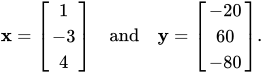
Consider two ⁠${\displaystyle n}$⁠-dimensional vectors that are formed as a list of ⁠${\displaystyle n}$⁠ scalars, such as the three-dimensional vectors $${\displaystyle \mathbf{x}=\left[\begin{array}{c}1\\ -3\\ 4\end{array}\right]\text{and}\mathbf{y}=\left[\begin{array}{c}-20\\ 60\\ -80\end{array}\right].}$$ These vectors are said to be scalar multiples of each other, or parallel, or collinear, if there is a scalar ⁠${\displaystyle \lambda }$⁠ such that $${\displaystyle \mathbf{y}=\lambda \mathbf{x}.}$$ In this example, ⁠${\displaystyle \lambda =-20}$⁠.

Now consider the linear transformation of ⁠${\displaystyle n}$⁠-dimensional vectors defined by an ⁠${\displaystyle n\times n}$⁠ matrix ⁠${\displaystyle A}$⁠: $${\displaystyle A\mathbf{v}=\mathbf{w},}$$ or $${\displaystyle \left[\begin{array}{cccc}{A}_{11}& A_{12}& \cdots & A_{1n}\\ A_{21}& A_{22}& \cdots & A_{2n}\\ ⋮& ⋮& \ddots & ⋮\\ A_{n1}& A_{n2}& \cdots & A_{nn}\end{array}\right]\left[\begin{array}{c}{v}_1\\ v_2\\ ⋮\\ v_n\end{array}\right]=\left[\begin{array}{c}{w}_1\\ w_2\\ ⋮\\ w_n\end{array}\right]}$$ where, for each row, $${\displaystyle w_i=A_{i1}{v}_1+A_{i2}{v}_2+\cdots +A_{in}{v}_n=\sum _{j=1}^n{A}_{ij}{v}_j.}$$

If it occurs that ⁠${\displaystyle \mathbf{v}}$⁠ and ⁠${\displaystyle \mathbf{w}}$⁠ are scalar multiples, that is, if

${\displaystyle A\mathbf{v}=\mathbf{w}=\lambda \mathbf{v}}$,

1

then ⁠${\displaystyle \mathbf{v}}$⁠ is an eigenvector of the linear transformation ⁠${\displaystyle A}$⁠ and the scale factor ⁠${\displaystyle \lambda }$⁠ is the eigenvalue corresponding to that eigenvector. Equation (1) is the eigenvalue equation for the matrix ⁠${\displaystyle A}$⁠.

Equation (1) can be stated equivalently as

${\displaystyle \left(A-\lambda I\right)\mathbf{v}=\mathbf{0}}$,

2

where ⁠${\displaystyle I}$⁠ is the ⁠${\displaystyle n\times n}$⁠ identity matrix and ⁠${\displaystyle \mathbf{0}}$⁠ is the zero vector.

Eigenvalues and characteristic polynomial

Main article: Characteristic polynomial

Equation (2) has a nonzero solution v if and only if the determinant of the matrix (A − λI) is zero. Therefore, the eigenvalues of A are values of λ that satisfy the equation

${\displaystyle det(A-\lambda I)=0}$.

3

Using the Leibniz formula for determinants, the left-hand side of equation (3) is a polynomial function of the variable λ and the degree of this polynomial is n, the order of the matrix A. Its coefficients depend on the entries of A, except that its term of degree n is always (−1)ⁿλⁿ. This polynomial is called the characteristic polynomial of A. Equation (3) is called the characteristic equation or secular equation of A.

The characteristic polynomial of an n-by-n matrix A, being a polynomial of degree n, has at most n complex number roots, which can be found by factoring the characteristic polynomial, or numerically by root finding. The characteristic polynomial can be factored into the product of n linear terms:

${\displaystyle det(A-\lambda I)=({\lambda }_1-\lambda )({\lambda }_2-\lambda )\cdots ({\lambda }_n-\lambda )}$,

4

where the complex numbers λ₁, λ₂, ..., λ_n, each of which is an eigenvalue, may repeat. (The number of times an eigenvalue appears in the characteristic polynomial is known as its algebraic multiplicity.)

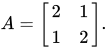
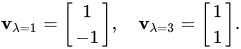
As a brief example, which is described in more detail in the examples section later, consider the matrix $${\displaystyle A=\left[\begin{array}{cc}2& 1\\ 1& 2\end{array}\right].}$$ Taking the determinant of (A − λI), the characteristic polynomial of A is $${\displaystyle det(A-\lambda I)=\left|\begin{array}{cc}2-\lambda & 1\\ 1& 2-\lambda \end{array}\right|=3-4\lambda +{\lambda }^2.}$$ Setting the characteristic polynomial equal to zero, it has roots at λ = 1 and λ = 3, which are the two eigenvalues of A. The eigenvectors corresponding to each eigenvalue λ can be found by solving for the components of v in the equation (A − λI)v = 0. In this example, the eigenvectors are any nonzero scalar multiples of $${\displaystyle {\mathbf{v}}_{\lambda =1}=\left[\begin{array}{c}1\\ -1\end{array}\right],{\mathbf{v}}_{\lambda =3}=\left[\begin{array}{c}1\\ 1\end{array}\right].}$$

If the entries of the matrix A are all real numbers, then the coefficients of the characteristic polynomial will also be real numbers, but the eigenvalues may still have nonzero imaginary parts. The entries of the corresponding eigenvectors therefore may also have nonzero imaginary parts. Similarly, the eigenvalues may be irrational numbers even if all the entries of A are rational numbers or even if they are all integers. However, if the entries of A are all algebraic numbers, which include the rationals, then the eigenvalues must also be algebraic numbers.

The non-real roots of a real polynomial with real coefficients can be grouped into pairs of complex conjugates, namely with the two members of each pair having imaginary parts that differ only in sign and the same real part. If the degree is odd, then by the intermediate value theorem at least one of the roots is real. Therefore, any real matrix with odd order has at least one real eigenvalue, whereas a real matrix with even order may not have any real eigenvalues. The eigenvectors associated with these complex eigenvalues are also complex and also appear in complex conjugate pairs.

Spectrum of a matrix

The spectrum of a matrix is the list of its eigenvalues, repeated according to their multiplicities; in a shorter notation, the set of its eigenvalues with their multiplicities indicated.

An important quantity associated with the spectrum of a matrix is the maximum absolute value of all of its eigenvalues. This is known as the spectral radius of the considered matrix.

Algebraic multiplicity

Let λ_i be an eigenvalue of an n-by-n matrix A. The algebraic multiplicity μ_A(λ_i) of the eigenvalue is its multiplicity as a root of the characteristic polynomial, that is, the largest integer k such that (λ_i − λ)^k evenly divides that polynomial.

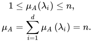
Suppose a matrix A has order n and d ≤ n distinct eigenvalues. Whereas equation (4) factors the characteristic polynomial of A into the product of n linear terms with some terms potentially repeating, the characteristic polynomial can also be written as the product of d terms each corresponding to a distinct eigenvalue and raised to the power of the algebraic multiplicity: $${\displaystyle det(A-\lambda I)=({\lambda }_1-\lambda {)}^{{\mu }_A({\lambda }_1)}({\lambda }_2-\lambda {)}^{{\mu }_A({\lambda }_2)}\cdots ({\lambda }_d-\lambda {)}^{{\mu }_A({\lambda }_d)}.}$$ If d = n, then the right-hand side is the product of n linear terms, and this is the same as equation (4). The size of each eigenvalue's algebraic multiplicity is related to the dimension n as $${\displaystyle \begin{array}{rl}1& \le {\mu }_A({\lambda }_i)\le n,\\ {\mu }_A& =\sum _{i=1}^d{\mu }_A\left({\lambda }_i\right)=n.\end{array}}$$ If μ_A(λ_i) = 1, then λ_i is said to be a simple eigenvalue. If μ_A(λ_i) equals the geometric multiplicity of λ_i (denoted by γ_A(λ_i) and defined in the next section), then λ_i is said to be a semisimple eigenvalue.

Eigenspaces, geometric multiplicities, and eigenbasis for a matrix

Given a particular eigenvalue ⁠${\displaystyle \lambda }$⁠ of the ⁠${\displaystyle n\times n}$⁠ matrix ⁠${\displaystyle A}$⁠, define the set ⁠${\displaystyle E}$⁠ to be all vectors ⁠${\displaystyle \mathbf{v}}$⁠ that satisfy equation (2): $${\displaystyle E=\left\{\mathbf{v}:\left(A-\lambda I\right)\mathbf{v}=\mathbf{0}\right\}.}$$ :\left(A-\lambda I\right)\mathbf {v} =\mathbf {0} \right\}.} On one hand, ⁠${\displaystyle E}$⁠ is precisely the kernel or nullspace of the matrix ⁠${\displaystyle A-\lambda I}$⁠. On the other hand, by definition, any nonzero vector that satisfies this condition is an eigenvector of ⁠${\displaystyle A}$⁠ associated with ⁠${\displaystyle \lambda }$⁠; so ⁠${\displaystyle E}$⁠ is the union of the zero vector with the set of all eigenvectors of ⁠${\displaystyle A}$⁠ associated with ⁠${\displaystyle \lambda }$⁠. The space ⁠${\displaystyle E}$⁠ is called the eigenspace or characteristic space of ⁠${\displaystyle A}$⁠ associated with ⁠${\displaystyle \lambda }$⁠. In general, ⁠${\displaystyle \lambda }$⁠ is a complex number and the eigenvectors are complex ⁠${\displaystyle n\times 1}$⁠ matrices (column vectors). Because every nullspace is a linear subspace of the domain, ⁠${\displaystyle E}$⁠ is a linear subspace of ⁠${\displaystyle {\mathbb{C}}^n}$⁠.

Because the eigenspace ⁠${\displaystyle E}$⁠ is a linear subspace, it is closed under addition. That is, if two vectors ⁠${\displaystyle \mathbf{u}}$⁠ and ⁠${\displaystyle \mathbf{v}}$⁠ belong to the set ⁠${\displaystyle E}$⁠, written ⁠${\displaystyle \mathbf{u},\mathbf{v}\in E}$⁠, then ⁠${\displaystyle \mathbf{u}+\mathbf{v}\in E}$⁠, or equivalently ⁠${\displaystyle A(\mathbf{u}+\mathbf{v})=\lambda (\mathbf{u}+\mathbf{v})}$⁠. This can be checked using the distributive property of matrix multiplication. Similarly, because ⁠${\displaystyle E}$⁠ is a linear subspace, it is closed under scalar multiplication. That is, if ⁠${\displaystyle \mathbf{v}\in E}$⁠ and ⁠${\displaystyle \alpha \in \mathbb{C}}$⁠, then ⁠${\displaystyle \alpha \mathbf{v}\in E}$⁠, or equivalently ⁠${\displaystyle A(\alpha \mathbf{v})=\lambda (\alpha \mathbf{v})}$⁠. This can be checked by noting that multiplication of complex matrices by complex numbers is commutative. As long as ⁠${\displaystyle \mathbf{u}+\mathbf{v}}$⁠ and ⁠${\displaystyle \alpha \mathbf{v}}$⁠ are not zero, they are also eigenvectors of ⁠${\displaystyle A}$⁠ associated with ⁠${\displaystyle \lambda }$⁠.

The dimension of the eigenspace ⁠${\displaystyle E}$⁠ associated with ⁠${\displaystyle \lambda }$⁠, or equivalently the maximum number of linearly independent eigenvectors associated with ⁠${\displaystyle \lambda }$⁠, is referred to as the eigenvalue's geometric multiplicity and denoted by ⁠${\displaystyle {\gamma }_A(\lambda )}$⁠. Because ⁠${\displaystyle E}$⁠ is also the nullspace of ⁠${\displaystyle A-\lambda I}$⁠, the geometric multiplicity of ⁠${\displaystyle \lambda }$⁠ is the dimension of the nullspace of ⁠${\displaystyle A-\lambda I}$⁠, also called the nullity of ⁠${\displaystyle A-\lambda I}$⁠. This quantity is related to the size and rank of ⁠${\displaystyle A-\lambda I}$⁠ by the equation: $${\displaystyle {\gamma }_A(\lambda )=n-\mathrm{rank}(A-\lambda I).}$$ Because of the definition of eigenvalues and eigenvectors, an eigenvalue's geometric multiplicity must be at least one, that is, each eigenvalue has at least one associated eigenvector. Furthermore, an eigenvalue's geometric multiplicity cannot exceed its algebraic multiplicity. Additionally, recall that an eigenvalue's algebraic multiplicity cannot exceed ⁠${\displaystyle n}$⁠. In summary, $${\displaystyle 1\le {\gamma }_A(\lambda )\le {\mu }_A(\lambda )\le n.}$$

Proof of inequality ⁠${\displaystyle {\gamma }_A(\lambda )\le {\mu }_A(\lambda )}$⁠: Let B = A − λI, where λ is a fixed complex number, and the eigenspace associated with λ is the nullspace of B. Let the dimension of that eigenspace be ⁠${\displaystyle k={\gamma }_A(\lambda )}$⁠. This means that the last k rows of the echelon form of B are zero. Thus, there is an invertible matrix E coming from Gauss-Jordan reduction, such that $${\displaystyle EB=\left[\begin{array}{cc}\ast & \ast \\ {\mathbf{0}}_{k\times (n-k)}& {\mathbf{0}}_{k\times k}\end{array}\right].}$$ Therefore the last k rows of EB − tE are (−t) times the last k rows of E. Therefore the polynomial t^k evenly divides the polynomial det(EB − tE), because of basic properties of determinants (homogeneity). On the other hand, det(EB − tE) = det E det(B − tI) = p_A(t + λ) det E, so (t − λ)^k divides p_A(t), and so the algebraic multiplicity of λ is at least ⁠${\displaystyle k}$⁠. Q.E.D.

Suppose A has d ≤ n distinct eigenvalues λ₁, ..., λ_d, where the geometric multiplicity of λ_i is γ_A(λ_i). The total geometric multiplicity of A, $${\displaystyle {\gamma }_A=\sum _{i=1}^d{\gamma }_A({\lambda }_i),}$$ is the dimension of the sum of all the eigenspaces of A's eigenvalues, or equivalently the maximum number of linearly independent eigenvectors of A. By construction, ⁠${\displaystyle d\le {\gamma }_A\le n}$⁠. If ⁠${\displaystyle {\gamma }_A=n}$⁠, then:

• The direct sum of the eigenspaces of all of A's eigenvalues is the entire vector space ⁠${\displaystyle {\mathbb{C}}^n}$⁠.
• A basis of ${\displaystyle {\mathbb{C}}^n}$ can be formed from n linearly independent eigenvectors of A; such a basis is called an eigenbasis.
• Any vector in ${\displaystyle {\mathbb{C}}^n}$ can be written as a linear combination of eigenvectors of A.

Additional properties

Let A be an arbitrary n × n matrix of complex numbers with eigenvalues λ₁, ..., λ_n. Each eigenvalue appears μ_A(λ_i) times in this list, where μ_A(λ_i) is the eigenvalue's algebraic multiplicity. The following are properties of this matrix and its eigenvalues:

• The trace of ⁠${\displaystyle A}$⁠, defined as the sum of its diagonal elements, is also the sum of all its eigenvalues: $${\displaystyle \mathrm{tr}(A)=\sum _{i=1}^n{a}_{ii}=\sum _{i=1}^n{\lambda }_i={\lambda }_1+{\lambda }_2+\cdots +{\lambda }_n.}$$
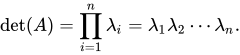
• The determinant of ⁠${\displaystyle A}$⁠ is the product of all its eigenvalues:$${\displaystyle det(A)=\prod _{i=1}^n{\lambda }_i={\lambda }_1{\lambda }_2\cdots {\lambda }_n.}$$
• For any positive integer ⁠${\displaystyle k}$⁠, the eigenvalues of the ⁠${\displaystyle k}$⁠th power of ⁠${\displaystyle A}$⁠, that is, ⁠${\displaystyle A^k}$⁠, are ⁠${\displaystyle {\lambda }_1^k,\dots ,{\lambda }_n^k}$⁠.
• The eigenvalues of matrix ⁠${\displaystyle A+I}$⁠ (where ⁠${\displaystyle I}$⁠ is the identity matrix) are ⁠${\displaystyle {\lambda }_1+1,\dots ,{\lambda }_n+1}$⁠. Moreover, for any ⁠${\displaystyle \alpha \in \mathbb{C}}$⁠, the eigenvalues of matrix ⁠${\displaystyle A+\alpha I}$⁠ are ⁠${\displaystyle {\lambda }_1+\alpha ,\dots ,{\lambda }_n+\alpha }$⁠.
• More generally, for any polynomial ⁠${\displaystyle P}$⁠, the eigenvalues of matrix ⁠${\displaystyle P(A)}$⁠ are ⁠${\displaystyle P({\lambda }_1),\dots ,P({\lambda }_n)}$⁠.
• ⁠${\displaystyle A}$⁠ is invertible if and only if every eigenvalue ⁠${\displaystyle {\lambda }_i}$⁠ is nonzero.
• If ⁠${\displaystyle A}$⁠ is invertible, then the eigenvalues of ⁠${\displaystyle A^{-1}}$⁠ are $\frac{1}{{\lambda }_1},\dots ,\frac{1}{{\lambda }_n}$ and for each pair of corresponding eigenvalues, the geometric multiplicities ⁠${\displaystyle {\gamma }_A({\lambda }_i)}$⁠ and ${\gamma }_{A^{-1}}(\frac{1}{{\lambda }_i})$ coincide. Moreover, since the characteristic polynomial of the inverse is the reciprocal polynomial of the original up to a scalar factor, for each pair of corresponding eigenvalues, the algebraic multiplicities ⁠${\displaystyle {\mu }_A({\lambda }_i)}$⁠ and ${\mu }_{A^{-1}}(\frac{1}{{\lambda }_i})$ coincide.
• If ⁠${\displaystyle A}$⁠ is equal to its conjugate transpose ⁠${\displaystyle A^{\ast }}$⁠, that is, ⁠${\displaystyle A}$⁠ is Hermitian, then every eigenvalue ⁠${\displaystyle {\lambda }_i}$⁠ is real. The same is true of any symmetric real matrix.
• If ⁠${\displaystyle A}$⁠ is not only Hermitian but also positive-definite, positive-semidefinite, negative-definite, or negative-semidefinite, then every eigenvalue ⁠${\displaystyle {\lambda }_i}$⁠ is positive, non-negative, negative, or non-positive, respectively.
• If ⁠${\displaystyle A}$⁠ is unitary, then every eigenvalue ⁠${\displaystyle {\lambda }_i}$⁠ has absolute value ⁠${\displaystyle |{\lambda }_i|=1}$⁠.

Left and right eigenvectors

See also: left and right (algebra)

Many disciplines traditionally represent vectors as matrices with a single column rather than as matrices with a single row. For that reason, the word "eigenvector" in the context of matrices almost always refers to a 'right eigenvector', namely a column vector that right multiplies the n × n matrix A in the defining equation, equation (1), $${\displaystyle A\mathbf{v}=\lambda \mathbf{v}.}$$ The eigenvalue and eigenvector problem can also be defined for row vectors that left multiply matrix A. In this formulation, the defining equation is $${\displaystyle \mathbf{u}A=\kappa \mathbf{u},}$$ where κ is a scalar and u is a 1 × n matrix. Any row vector u satisfying this equation is called a 'left eigenvector' of A, and κ is still called its associated eigenvalue. Taking the transpose of this equation, $${\displaystyle A^{\mathsf{T}}{\mathbf{u}}^{\mathsf{T}}=\kappa {\mathbf{u}}^{\mathsf{T}}.}$$

Comparing this equation to equation (1), it follows immediately that a left eigenvector of ⁠${\displaystyle A}$⁠ is the same as the transpose of a right eigenvector of ⁠${\displaystyle A^{\mathsf{T}}}$⁠, with the same eigenvalue. Furthermore, since the characteristic polynomial of ⁠${\displaystyle A^{\mathsf{T}}}$⁠ is the same as the characteristic polynomial of ⁠${\displaystyle A}$⁠, the left and right eigenvectors of ⁠${\displaystyle A}$⁠ are associated with the same eigenvalues.

Eigenvalues of transpose

A matrix has the same eigenvalues as its transpose, as can be directly seen as follows. Assume ⁠${\displaystyle \lambda }$⁠ is an eigenvalue of an ⁠${\displaystyle n\times n}$⁠ matrix ⁠${\displaystyle A}$⁠ with eigenvector ⁠${\displaystyle x}$⁠. Then ⁠${\displaystyle Ax=\lambda x}$⁠; equivalently, ⁠${\displaystyle (A-\lambda I)x=0}$⁠.

Thus, the columns of ⁠${\displaystyle (A-\lambda I)}$⁠ are linearly dependent. Equivalently, the rank of the matrix is less than ⁠${\displaystyle n}$⁠.

But as column rank = row rank, the rows are also linearly dependent. Hence, there are numbers ⁠${\displaystyle y_1,y_2,\dots ,y_n}$⁠, not all zero, such that $\sum _{i=1}^{i=n}{y}_i{R}_i=0,$ where the ⁠${\displaystyle R_i}$⁠'s are the rows of ⁠${\displaystyle (A-\lambda I)}$⁠. Let the row vector ⁠${\displaystyle y=(y_1,y_2,\dots ,y_n)}$⁠; then ⁠${\displaystyle y(A-\lambda I)=0}$⁠. Taking the transpose, ⁠${\displaystyle (A^{\mathsf{T}}-\lambda I)y^{\mathsf{T}}=0}$⁠. Moreover, ⁠${\displaystyle y^{\mathsf{T}}}$⁠ is not the zero vector; so ⁠${\displaystyle \lambda }$⁠ is also an eigenvalue of ⁠${\displaystyle A^{\mathsf{T}}}$⁠.

Furthermore, this argument shows that the eigenvalues of ${\displaystyle A}$ and ${\displaystyle A^{\mathsf{T}}}$ have the same geometric multiplicity (since column nullity = row nullity).

Diagonalization and eigendecomposition

Main article: Eigendecomposition of a matrix

Suppose the eigenvectors of A form a basis of ⁠${\displaystyle {\mathbb{C}}^n}$⁠, or equivalently A has n linearly independent eigenvectors v₁, v₂, ..., v_n (with associated eigenvalues λ₁, λ₂, ..., λ_n). The eigenvectors need not be orthogonal to one another, and the eigenvalues need not be distinct. Define the square matrix Q whose columns are the n linearly independent eigenvectors of A, $${\displaystyle Q=\left[\begin{array}{cccc}{\mathbf{v}}_1& {\mathbf{v}}_2& \cdots & {\mathbf{v}}_n\end{array}\right].}$$ Since each column of Q is an eigenvector of A, right multiplying A by Q scales each column of Q by its associated eigenvalue: $${\displaystyle AQ=\left[\begin{array}{cccc}{\lambda }_1{\mathbf{v}}_1& {\lambda }_2{\mathbf{v}}_2& \cdots & {\lambda }_n{\mathbf{v}}_n\end{array}\right].}$$

With this in mind, define the diagonal matrix Λ where each diagonal element Λ_ii is the eigenvalue associated with the ith column of Q. Then $${\displaystyle AQ=Q\Lambda .}$$ Because the columns of Q are linearly independent, Q is invertible. Right multiplying both sides of the equation by Q⁻¹, $${\displaystyle A=Q\Lambda Q^{-1};}$$ or instead left multiplying both sides by Q⁻¹, $${\displaystyle Q^{-1}AQ=\Lambda .}$$ A can therefore be decomposed into a matrix composed of its eigenvectors, a diagonal matrix with its eigenvalues along the diagonal, and the inverse of the matrix of eigenvectors. This is called the eigendecomposition; it is a similarity transformation. Such a matrix A is said to be similar to the diagonal matrix Λ, or diagonalizable. The matrix Q is the change of basis matrix of the similarity transformation. Essentially, the matrices A and Λ represent the same linear transformation expressed in two different bases. The eigenvectors are used as the basis when representing the linear transformation as Λ.

Conversely, suppose a matrix A is diagonalizable. Let P be a non-singular square matrix such that P⁻¹AP is some diagonal matrix D. Left multiplying both by P yields AP = PD. Each column of P must therefore be an eigenvector of A whose eigenvalue is the corresponding diagonal element of D. Since the columns of P must be linearly independent for P to be invertible, there exist n linearly independent eigenvectors of A.

In conclusion, the eigenvectors of ⁠${\displaystyle A}$⁠ form a basis of ⁠${\displaystyle {\mathbb{C}}^n}$⁠ if and only if ⁠${\displaystyle A}$⁠ is diagonalizable.

A matrix that is not diagonalizable is said to be defective. For defective matrices, the notion of eigenvectors generalizes to generalized eigenvectors and the diagonal matrix of eigenvalues generalizes to the Jordan normal form. Over an algebraically closed field, any matrix A has a Jordan normal form and therefore admits a basis of generalized eigenvectors and a decomposition into generalized eigenspaces.

Variational characterization

Main article: Min-max theorem

In the Hermitian case, eigenvalues can be given a variational characterization. The largest eigenvalue of H is the maximum value of the quadratic form x^THx/x^Tx. A value of x that realizes that maximum is an eigenvector.

Matrix examples

Two-dimensional matrix example

The transformation matrix A =  ⎡⎣²
₁ ¹
₂⎤⎦   preserves the direction of magenta vectors parallel to v_λ=1 = [1 −1]^T and blue vectors parallel to v_λ=3 = [1 1]^T. The red vectors are not parallel to either eigenvector, so, their directions are changed by the transformation. The lengths of the magenta vectors are unchanged after the transformation (due to their eigenvalue of 1), while blue vectors are three times the length of the original (due to their eigenvalue of 3). See also: An extended version, showing all four quadrants.

Consider the matrix $${\displaystyle A=\left[\begin{array}{cc}2& 1\\ 1& 2\end{array}\right].}$$ The figure on the right shows the effect of this transformation on point coordinates in the plane. The eigenvectors v of this transformation satisfy equation (1), and the values of λ for which the determinant of the matrix (A − λI) equals zero are the eigenvalues.

Taking the determinant to find characteristic polynomial of A, $${\displaystyle \begin{array}{rl}det(A-\lambda I)& =\left|\left[\begin{array}{cc}2& 1\\ 1& 2\end{array}\right]-\lambda \left[\begin{array}{cc}1& 0\\ 0& 1\end{array}\right]\right|=\left|\begin{array}{cc}2-\lambda & 1\\ 1& 2-\lambda \end{array}\right|\\ & =3-4\lambda +{\lambda }^2\\ & =(\lambda -3)(\lambda -1).\end{array}}$$ Setting the characteristic polynomial equal to zero, it has roots at λ = 1 and λ = 3, which are the two eigenvalues of A.

For λ = 1, equation (2) becomes, $${\displaystyle \begin{array}{rl}(A-I){\mathbf{v}}_{\lambda =1}& =\left[\begin{array}{cc}1& 1\\ 1& 1\end{array}\right]\left[\begin{array}{c}{v}_1\\ v_2\end{array}\right]=\left[\begin{array}{c}0\\ 0\end{array}\right]\\ 1v_1+1v_2& =0\end{array}}$$ Any nonzero vector with v₁ = −v₂ solves this equation. Therefore, $${\displaystyle {\mathbf{v}}_{\lambda =1}=\left[\begin{array}{c}{v}_1\\ -v_1\end{array}\right]=\left[\begin{array}{c}1\\ -1\end{array}\right]}$$ is an eigenvector of A corresponding to λ = 1, as is any scalar multiple of this vector.

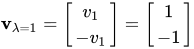
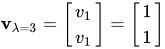
For λ = 3, equation (2) becomes $${\displaystyle \begin{array}{rl}(A-3I){\mathbf{v}}_{\lambda =3}& =\left[\begin{array}{cc}-1& \phantom{}1\\ \phantom{}1& -1\end{array}\right]\left[\begin{array}{c}{v}_1\\ v_2\end{array}\right]=\left[\begin{array}{c}0\\ 0\end{array}\right]\\ -1v_1+1v_2& =0;\\ 1v_1-1v_2& =0\end{array}}$$ Any nonzero vector with v₁ = v₂ solves this equation. Therefore, $${\displaystyle {\mathbf{v}}_{\lambda =3}=\left[\begin{array}{c}{v}_1\\ v_1\end{array}\right]=\left[\begin{array}{c}1\\ 1\end{array}\right]}$$ is an eigenvector of A corresponding to λ = 3, as is any scalar multiple of this vector. Thus, the vectors v_λ=1 and v_λ=3 are eigenvectors of A associated with the eigenvalues λ = 1 and λ = 3, respectively.

Three-dimensional matrix example

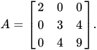
Consider the matrix $${\displaystyle A=\left[\begin{array}{ccc}2& 0& 0\\ 0& 3& 4\\ 0& 4& 9\end{array}\right].}$$ The characteristic polynomial of A is $${\displaystyle \begin{array}{rl}det(A-\lambda I)& =\left|\left[\begin{array}{ccc}2& 0& 0\\ 0& 3& 4\\ 0& 4& 9\end{array}\right]-\lambda \left[\begin{array}{ccc}1& 0& 0\\ 0& 1& 0\\ 0& 0& 1\end{array}\right]\right|=\left|\begin{array}{ccc}2-\lambda & 0& 0\\ 0& 3-\lambda & 4\\ 0& 4& 9-\lambda \end{array}\right|,\\ & =(2-\lambda )[(3-\lambda )(9-\lambda )-16]=-{\lambda }^3+14{\lambda }^2-35\lambda +22.\end{array}}$$

The roots of the characteristic polynomial are 2, 1, and 11, which are the only three eigenvalues of A. These eigenvalues correspond to the eigenvectors [1 0 0]^T, [0 −2 1]^T, and [0 1 2]^T, or any nonzero multiple thereof.

Three-dimensional matrix example with complex eigenvalues

Consider the cyclic permutation matrix $${\displaystyle A=\left[\begin{array}{ccc}0& 1& 0\\ 0& 0& 1\\ 1& 0& 0\end{array}\right].}$$

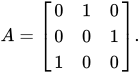
This matrix shifts the coordinates of the vector up by one position and moves the first coordinate to the bottom. Its characteristic polynomial is 1 − λ³, whose roots are $${\displaystyle \begin{array}{rl}{\lambda }_1& =1\\ {\lambda }_2& =-\frac{1}{2}+i\frac{\sqrt{3}}{2}\\ {\lambda }_3& ={\lambda }_2^{\ast }=-\frac{1}{2}-i\frac{\sqrt{3}}{2}\end{array}}$$ where i is an imaginary unit with i² = −1.

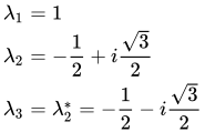
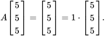
For the real eigenvalue λ₁ = 1, any vector with three equal nonzero entries is an eigenvector. For example, $${\displaystyle A\left[\begin{array}{c}5\\ 5\\ 5\end{array}\right]=\left[\begin{array}{c}5\\ 5\\ 5\end{array}\right]=1\cdot \left[\begin{array}{c}5\\ 5\\ 5\end{array}\right].}$$

For the complex conjugate pair of imaginary eigenvalues, $${\displaystyle {\lambda }_2{\lambda }_3=1,{\lambda }_2^2={\lambda }_3,{\lambda }_3^2={\lambda }_2.}$$ Then $${\displaystyle A\left[\begin{array}{c}1\\ {\lambda }_2\\ {\lambda }_3\end{array}\right]=\left[\begin{array}{c}{\lambda }_2\\ {\lambda }_3\\ 1\end{array}\right]={\lambda }_2\cdot \left[\begin{array}{c}1\\ {\lambda }_2\\ {\lambda }_3\end{array}\right],}$$ and $${\displaystyle A\left[\begin{array}{c}1\\ {\lambda }_3\\ {\lambda }_2\end{array}\right]=\left[\begin{array}{c}{\lambda }_3\\ {\lambda }_2\\ 1\end{array}\right]={\lambda }_3\cdot \left[\begin{array}{c}1\\ {\lambda }_3\\ {\lambda }_2\end{array}\right].}$$

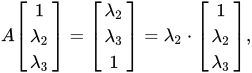
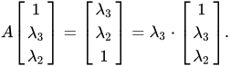
Therefore, the other two eigenvectors of A are complex and are v_λ2 = [1 λ₂ λ₃]^T and v_λ3 = [1 λ₃ λ₂]^T with eigenvalues λ₂ and λ₃, respectively. The two complex eigenvectors also appear in a complex conjugate pair, $${\displaystyle {\mathbf{v}}_{{\lambda }_2}={\mathbf{v}}_{{\lambda }_3}^{\ast }.}$$

Diagonal matrix example

Matrices with entries only along the main diagonal are called diagonal matrices. The eigenvalues of a diagonal matrix are the diagonal elements themselves. Consider the matrix $${\displaystyle A=\left[\begin{array}{ccc}1& 0& 0\\ 0& 2& 0\\ 0& 0& 3\end{array}\right].}$$ The characteristic polynomial of A is $${\displaystyle det(A-\lambda I)=(1-\lambda )(2-\lambda )(3-\lambda ),}$$ which has the roots λ₁ = 1, λ₂ = 2, and λ₃ = 3. These roots are the diagonal elements as well as the eigenvalues of A.

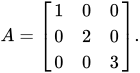
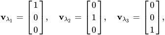
Each diagonal element corresponds to an eigenvector whose only nonzero component is in the same row as that diagonal element. In the example, the eigenvalues correspond to the eigenvectors, $${\displaystyle {\mathbf{v}}_{{\lambda }_1}=\left[\begin{array}{c}1\\ 0\\ 0\end{array}\right],{\mathbf{v}}_{{\lambda }_2}=\left[\begin{array}{c}0\\ 1\\ 0\end{array}\right],{\mathbf{v}}_{{\lambda }_3}=\left[\begin{array}{c}0\\ 0\\ 1\end{array}\right],}$$ respectively, as well as scalar multiples of these vectors.

Triangular matrix example

A matrix whose elements above the main diagonal are all zero is called a lower triangular matrix, while a matrix whose elements below the main diagonal are all zero is called an upper triangular matrix. As with diagonal matrices, the eigenvalues of triangular matrices are the elements of the main diagonal.

Consider the lower triangular matrix, $${\displaystyle A=\left[\begin{array}{ccc}1& 0& 0\\ 1& 2& 0\\ 2& 3& 3\end{array}\right].}$$

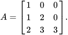
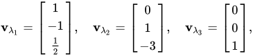
The characteristic polynomial of A is $${\displaystyle det(A-\lambda I)=(1-\lambda )(2-\lambda )(3-\lambda ),}$$ which has the roots λ₁ = 1, λ₂ = 2, and λ₃ = 3. These roots are the diagonal elements as well as the eigenvalues of A.

These eigenvalues correspond to the eigenvectors, $${\displaystyle {\mathbf{v}}_{{\lambda }_1}=\left[\begin{array}{c}1\\ -1\\ \frac{1}{2}\end{array}\right],{\mathbf{v}}_{{\lambda }_2}=\left[\begin{array}{c}0\\ 1\\ -3\end{array}\right],{\mathbf{v}}_{{\lambda }_3}=\left[\begin{array}{c}0\\ 0\\ 1\end{array}\right],}$$ respectively, as well as scalar multiples of these vectors.

Matrix with repeated eigenvalues example

As in the previous example, the lower triangular matrix $${\displaystyle A=\left[\begin{array}{cccc}2& 0& 0& 0\\ 1& 2& 0& 0\\ 0& 1& 3& 0\\ 0& 0& 1& 3\end{array}\right],}$$ has a characteristic polynomial that is the product of its diagonal elements, $${\displaystyle det(A-\lambda I)=\left|\begin{array}{cccc}2-\lambda & 0& 0& 0\\ 1& 2-\lambda & 0& 0\\ 0& 1& 3-\lambda & 0\\ 0& 0& 1& 3-\lambda \end{array}\right|=(2-\lambda {)}^2(3-\lambda {)}^2.}$$

The roots of this polynomial, and hence the eigenvalues, are 2 and 3. The algebraic multiplicity of each eigenvalue is 2; in other words they are both double roots. The sum of the algebraic multiplicities of all distinct eigenvalues is μ_A = 4 = n, the order of the characteristic polynomial and the dimension of A.

On the other hand, the geometric multiplicity of the eigenvalue 2 is only 1, because its eigenspace is spanned by just one vector [0 1 −1 1]^T and is therefore 1-dimensional. Similarly, the geometric multiplicity of the eigenvalue 3 is 1 because its eigenspace is spanned by just one vector [0 0 0 1]^T. The total geometric multiplicity γ_A is 2, which is the smallest it could be for a matrix with two distinct eigenvalues. Geometric multiplicities are defined in a later section.

Eigenvector-eigenvalue identity

For a Hermitian matrix A, the norm squared of the αth component of a normalized eigenvector can be calculated using only the matrix eigenvalues and the eigenvalues of the corresponding minor matrix, $${\displaystyle |v_{i\alpha }{|}^2=\frac{\prod _k({\lambda }_i(A)-{\lambda }_k(A_{\alpha }))}{\prod _{k\ne i}({\lambda }_i(A)-{\lambda }_k(A))},}$$ where ⁠${\displaystyle A_{\alpha }}$⁠ is the submatrix formed by removing the αth row and column from the original matrix. This identity also extends to diagonalizable matrices. It has been discovered in and rediscovered many times in the literature.

Eigenvalues and eigenfunctions of differential operators

Main article: Eigenfunction

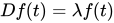
The definitions of eigenvalue and eigenvectors of a linear transformation T remains valid even if the underlying vector space is an infinite-dimensional Hilbert or Banach space. A widely used class of linear transformations acting on infinite-dimensional spaces are the differential operators on function spaces. Let D be a linear differential operator on the space ${\displaystyle C^{\mathrm{\infty }}(\mathbb{R})}$ of infinitely differentiable real functions of a real argument t. The eigenvalue equation for D is the differential equation $${\displaystyle Df(t)=\lambda f(t)}$$ The functions that satisfy this equation are eigenvectors of D and are commonly called 'eigenfunctions'.

Derivative operator example

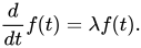
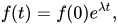
Consider the derivative operator ${\displaystyle \frac{d}{dt}}$ with eigenvalue equation $${\displaystyle \frac{d}{dt}f(t)=\lambda f(t).}$$ This differential equation can be solved by multiplying both sides by dt/f(t) and integrating. Its solution, the exponential function $${\displaystyle f(t)=f(0)e^{\lambda t},}$$ is the eigenfunction of the derivative operator. In this case the eigenfunction is itself a function of its associated eigenvalue. In particular, for λ = 0 the eigenfunction f(t) is a constant.

General definition

The concept of eigenvalues and eigenvectors extends naturally to arbitrary linear transformations on arbitrary vector spaces. Let V be any vector space over some field K of scalars, and let T be a linear transformation mapping V into V, $${\displaystyle T:V\to V.}$$

We say that a nonzero vector v ∈ V is an 'eigenvector' of T if and only if there exists a scalar λ ∈ K such that

${\displaystyle T(\mathbf{v})=\lambda \mathbf{v}.}$

5

This equation is called the eigenvalue equation for T, and the scalar λ is the eigenvalue of T corresponding to the eigenvector v. T(v) is the result of applying the transformation T to the vector v, while λv is the product of the scalar λ with v.

Eigenspaces, geometric multiplicity, and the eigenbasis

Given an eigenvalue λ, consider the set $${\displaystyle E=\left\{\mathbf{v}:T(\mathbf{v})=\lambda \mathbf{v}\right\},}$$ which is the union of the zero vector with the set of all eigenvectors associated with λ. E is called the eigenspace or characteristic space of T associated with λ. It is the kernel of the linear transformation T − λI.

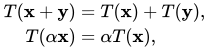
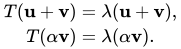
By definition of a linear transformation, $${\displaystyle \begin{array}{rl}T(\mathbf{x}+\mathbf{y})& =T(\mathbf{x})+T(\mathbf{y}),\\ T(\alpha \mathbf{x})& =\alpha T(\mathbf{x}),\end{array}}$$ for x, y ∈ V and α ∈ K. Therefore, if u and v are eigenvectors of T associated with eigenvalue λ, namely u, v ∈ E, then $${\displaystyle \begin{array}{rl}T(\mathbf{u}+\mathbf{v})& =\lambda (\mathbf{u}+\mathbf{v}),\\ T(\alpha \mathbf{v})& =\lambda (\alpha \mathbf{v}).\end{array}}$$ So, both u + v and αv are either zero or eigenvectors of T associated with λ, namely u + v, αv ∈ E, and E is closed under addition and scalar multiplication. The eigenspace E associated with λ is therefore a linear subspace of V. If that subspace has dimension 1, it is sometimes called an eigenline.

The geometric multiplicity γ_T(λ) of an eigenvalue λ is the dimension of the eigenspace associated with λ; that is, the maximum number of linearly independent eigenvectors associated with that eigenvalue. By the definition of eigenvalues and eigenvectors, γ_T(λ) ≥ 1 because every eigenvalue has at least one eigenvector.

The eigenspaces of T always form a direct sum. As a consequence, eigenvectors of different eigenvalues are always linearly independent. Therefore, the sum of the dimensions of the eigenspaces cannot exceed the dimension n of the vector space on which T operates, and there cannot be more than n distinct eigenvalues.

Any subspace spanned by eigenvectors of T is an invariant subspace of T, and the restriction of T to such a subspace is diagonalizable. Moreover, if the entire vector space V can be spanned by the eigenvectors of T, or equivalently if the direct sum of the eigenspaces associated with all the eigenvalues of T is the entire vector space V, then a basis of V called an eigenbasis can be formed from linearly independent eigenvectors of T. When T admits an eigenbasis, T is diagonalizable.

Spectral theory

Main article: Spectral theory

If λ is an eigenvalue of T, then the operator (T − λI) is not one-to-one, and therefore its inverse (T − λI)⁻¹ does not exist. The converse is true for finite-dimensional vector spaces, but not for infinite-dimensional vector spaces. In general, the operator (T − λI) may not have an inverse even if λ is not an eigenvalue.

For this reason, in functional analysis eigenvalues can be generalized to the spectrum of a linear operator T as the set of all scalars λ for which the operator (T − λI) has no bounded inverse. The spectrum of an operator always contains all its eigenvalues but is not limited to them.

Associative algebras and representation theory

Main article: Weight (representation theory)

One can generalize the algebraic object that is acting on the vector space, replacing a single operator acting on a vector space with an algebra representation – an associative algebra acting on a module. The study of such actions is the field of representation theory.

The representation-theoretical concept of weight is an analog of eigenvalues, while weight vectors and weight spaces are the analogs of eigenvectors and eigenspaces, respectively.

Hecke eigensheaf is a tensor-multiple of itself and is considered in Langlands correspondence.

Dynamic equations

The simplest difference equations have the form $${\displaystyle x_t=a_1{x}_{t-1}+a_2{x}_{t-2}+\cdots +a_k{x}_{t-k}.}$$ The solution of this equation for x in terms of t is found by using its characteristic equation $${\displaystyle {\lambda }^k-a_1{\lambda }^{k-1}-a_2{\lambda }^{k-2}-\cdots -a_{k-1}\lambda -a_k=0,}$$ which can be found by stacking into matrix form a set of equations consisting of the above difference equation and the k – 1 equations x_t–1 = x_t–1, ..., x_t–k+1 = x_t–k+1, giving a k-dimensional system of the first order in the stacked variable vector [x_t  ⋅⋅⋅  x_t–k+1] in terms of its once-lagged value, and taking the characteristic equation of this system's matrix. This equation gives k characteristic roots λ₁, ... , λ_k, for use in the solution equation $${\displaystyle x_t=c_1{\lambda }_1^t+\cdots +c_k{\lambda }_k^t.}$$

A similar procedure is used for solving a differential equation of the form $${\displaystyle \frac{d^{k}x}{d{t}^k}+a_{k-1}\frac{d^{k-1}x}{d{t}^{k-1}}+\cdots +a_1\frac{dx}{dt}+a_{0}x=0.}$$

Calculation

Main article: Eigenvalue algorithm

The calculation of eigenvalues and eigenvectors is a topic where theory, as presented in elementary linear algebra textbooks, is often very far from practice.

Classical method

The classical method is to first find the eigenvalues, and then calculate the eigenvectors for each eigenvalue. It is in several ways poorly suited for non-exact arithmetics such as floating-point.

Eigenvalues

The eigenvalues of a matrix A can be determined by finding the roots of the characteristic polynomial. This is easy for 2 × 2 matrices, but the difficulty increases rapidly with the size of the matrix.

In theory, the coefficients of the characteristic polynomial can be computed exactly, since they are sums of products of matrix elements; and there are algorithms that can find all the roots of a polynomial of arbitrary degree to any required accuracy. However, this approach is not viable in practice because the coefficients would be contaminated by unavoidable round-off errors, and the roots of a polynomial can be an extremely sensitive function of the coefficients (as exemplified by Wilkinson's polynomial). Even for matrices whose elements are integers the calculation becomes nontrivial, because the sums are very long; the constant term is the determinant, which for an n × n matrix is a sum of n! different products.

Explicit algebraic formulas for the roots of a polynomial exist only if the degree n is 4 or less. According to the Abel–Ruffini theorem there is no general, explicit and exact algebraic formula for the roots of a polynomial with degree 5 or more. (Generality matters because any polynomial with degree n is the characteristic polynomial of some companion matrix of order n.) Therefore, for matrices of order 5 or more, the eigenvalues and eigenvectors cannot be obtained by an explicit algebraic formula, and must therefore be computed by approximate numerical methods. Even the exact formula for the roots of a degree 3 polynomial is numerically impractical.

Eigenvectors

Once the (exact) value of an eigenvalue is known, the corresponding eigenvectors can be found by finding nonzero solutions of the eigenvalue equation, that becomes a system of linear equations with known coefficients. For example, once it is known that 6 is an eigenvalue of the matrix $${\displaystyle A=\left[\begin{array}{cc}4& 1\\ 6& 3\end{array}\right]}$$ we can find its eigenvectors by solving the equation Av = 6v, that is $${\displaystyle \left[\begin{array}{cc}4& 1\\ 6& 3\end{array}\right]\left[\begin{array}{c}x\\ y\end{array}\right]=6\cdot \left[\begin{array}{c}x\\ y\end{array}\right]}$$ This matrix equation is equivalent to two linear equations $${\displaystyle \{\begin{array}{rl}4x+\phantom{\mathrm{}}y& =6x\\ 6x+3y& =6y\end{array}}$$ that is, $${\displaystyle \{\begin{array}{rl}-2x+\phantom{\mathrm{}}y& =0\\ 6x-3y& =0\end{array}}$$

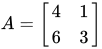
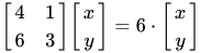
Both equations reduce to the single linear equation y = 2x. Therefore, any vector of the form [a  2a]^T, for any nonzero real number a, is an eigenvector of A with eigenvalue λ = 6.

The matrix A above has another eigenvalue λ = 1. A similar calculation shows that the corresponding eigenvectors are the nonzero solutions of 3x + y = 0, that is, any vector of the form [b  −3b]^T, for any nonzero real number b.

Simple iterative methods

Main article: Power iteration

The converse approach, of first seeking the eigenvectors and then determining each eigenvalue from its eigenvector, turns out to be far more tractable for computers. The easiest algorithm here consists of picking an arbitrary starting vector and then repeatedly multiplying it with the matrix (optionally normalizing the vector to keep its elements of reasonable size); this makes the vector converge towards an eigenvector. A variation is to instead multiply the vector by (A − μI)⁻¹; this causes it to converge to an eigenvector of the eigenvalue closest to ${\displaystyle \mu \in \mathbb{C}}$.

If v is (a good approximation of) an eigenvector of A, then the corresponding eigenvalue can be computed as $${\displaystyle \lambda =\frac{{\mathbf{v}}^{\ast }A\mathbf{v}}{{\mathbf{v}}^{\ast }\mathbf{v}}}$$ where v^∗ denotes the conjugate transpose of v.

Modern methods

Efficient, accurate methods to compute eigenvalues and eigenvectors of arbitrary matrices were not known until the QR algorithm was designed in 1961. Combining the Householder transformation with the LU decomposition results in an algorithm with better convergence than the QR algorithm. For large Hermitian sparse matrices, the Lanczos algorithm is one example of an efficient iterative method to compute eigenvalues and eigenvectors, among several other possibilities.

Most numeric methods that compute the eigenvalues of a matrix also determine a set of corresponding eigenvectors as a by-product of the computation, although sometimes implementors choose to discard the eigenvector information as soon as it is no longer needed.

Applications

Geometric transformations

Eigenvectors and eigenvalues can be useful for understanding linear transformations of geometric shapes. The following table presents some example transformations in the plane along with their 2 × 2 matrices, eigenvalues, and eigenvectors.

Eigenvalues of geometric transformations

	Scaling	Unequal scaling	Rotation	Horizontal shear	Hyperbolic rotation
Illustration
Matrix	${\displaystyle \left[\begin{array}{cc}k& 0\\ 0& k\end{array}\right]}$	${\displaystyle \left[\begin{array}{cc}{k}_1& 0\\ 0& k_2\end{array}\right]}$	${\displaystyle \left[\begin{array}{cc}\cos \theta & -\sin \theta \\ \sin \theta & \cos \theta \end{array}\right]}$	${\displaystyle \left[\begin{array}{cc}1& k\\ 0& 1\end{array}\right]}$	${\displaystyle \left[\begin{array}{cc}\cosh \phi & \sinh \phi \\ \sinh \phi & \cosh \phi \end{array}\right]}$
Characteristic polynomial	${\displaystyle (\lambda -k{)}^2}$	${\displaystyle (\lambda -k_1)(\lambda -k_2)}$	${\displaystyle {\lambda }^2-2\cos (\theta )\lambda +1}$	${\displaystyle (\lambda -1{)}^2}$	${\displaystyle {\lambda }^2-2\cosh (\phi )\lambda +1}$
Eigenvalues, ${\displaystyle {\lambda }_i}$	${\displaystyle {\lambda }_1={\lambda }_2=k}$	${\displaystyle \begin{array}{rl}{\lambda }_1& =k_1\\ {\lambda }_2& =k_2\end{array}}$	${\displaystyle \begin{array}{rl}{\lambda }_1& =e^{i\theta }\\ & =\cos \theta +i\sin \theta \\ {\lambda }_2& =e^{-i\theta }\\ & =\cos \theta -i\sin \theta \end{array}}$	${\displaystyle {\lambda }_1={\lambda }_2=1}$	${\displaystyle \begin{array}{rl}{\lambda }_1& =e^{\phi }\\ & =\cosh \phi +\sinh \phi \\ {\lambda }_2& =e^{-\phi }\\ & =\cosh \phi -\sinh \phi \end{array}}$
Algebraic mult., ${\displaystyle {\mu }_i=\mu ({\lambda }_i)}$	${\displaystyle {\mu }_1=2}$	${\displaystyle \begin{array}{rl}{\mu }_1& =1\\ {\mu }_2& =1\end{array}}$	${\displaystyle \begin{array}{rl}{\mu }_1& =1\\ {\mu }_2& =1\end{array}}$	${\displaystyle {\mu }_1=2}$	${\displaystyle \begin{array}{rl}{\mu }_1& =1\\ {\mu }_2& =1\end{array}}$
Geometric mult., ${\displaystyle {\gamma }_i=\gamma ({\lambda }_i)}$	${\displaystyle {\gamma }_1=2}$	${\displaystyle \begin{array}{rl}{\gamma }_1& =1\\ {\gamma }_2& =1\end{array}}$	${\displaystyle \begin{array}{rl}{\gamma }_1& =1\\ {\gamma }_2& =1\end{array}}$	${\displaystyle {\gamma }_1=1}$	${\displaystyle \begin{array}{rl}{\gamma }_1& =1\\ {\gamma }_2& =1\end{array}}$
Eigenvectors	All nonzero vectors	${\displaystyle \begin{array}{rl}{\mathbf{u}}_1& =\left[\begin{array}{c}1\\ 0\end{array}\right]\\ {\mathbf{u}}_2& =\left[\begin{array}{c}0\\ 1\end{array}\right]\end{array}}$	${\displaystyle \begin{array}{rl}{\mathbf{u}}_1& =\left[\begin{array}{c}1\\ -i\end{array}\right]\\ {\mathbf{u}}_2& =\left[\begin{array}{c}1\\ +i\end{array}\right]\end{array}}$	${\displaystyle {\mathbf{u}}_1=\left[\begin{array}{c}1\\ 0\end{array}\right]}$	${\displaystyle \begin{array}{rl}{\mathbf{u}}_1& =\left[\begin{array}{c}1\\ 1\end{array}\right]\\ {\mathbf{u}}_2& =\left[\begin{array}{c}1\\ -1\end{array}\right]\end{array}}$

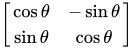
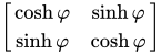
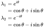
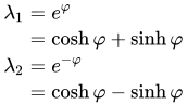
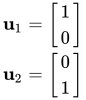
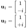
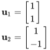
The characteristic equation for a rotation is a quadratic equation with discriminant D = −4(sin θ)², which is a negative number whenever θ is not an integer multiple of π (180°). Therefore, except for these special cases, the two eigenvalues are complex numbers, cos θ ± isin θ; and all eigenvectors have non-real entries. Indeed, except for those special cases, a rotation changes the direction of every nonzero vector in the plane.

A linear transformation that takes a square to a rectangle of the same area (a squeeze mapping) has reciprocal eigenvalues.

Principal component analysis

PCA of the multivariate Gaussian distribution centered at (1, 3) with a standard deviation of 3 in roughly the (0.878, 0.478) direction and of 1 in the orthogonal direction. The vectors shown are unit eigenvectors of the (symmetric, positive-semidefinite) covariance matrix scaled by the square root of the corresponding eigenvalue. Just as in the one-dimensional case, the square root is taken because the standard deviation is more readily visualized than the variance.

Main article: Principal component analysis

See also: Positive semidefinite matrix and Factor analysis

The eigendecomposition of a symmetric positive semidefinite (PSD) matrix yields an orthogonal basis of eigenvectors, each of which has a nonnegative eigenvalue. The orthogonal decomposition of a PSD matrix is used in multivariate analysis, where the sample covariance matrices are PSD. This orthogonal decomposition is called principal component analysis (PCA) in statistics. PCA studies linear relations among variables. PCA is performed on the covariance matrix or the correlation matrix (in which each variable is scaled to have its sample variance equal to one). For the covariance or correlation matrix, the eigenvectors correspond to principal components and the eigenvalues to the variance explained by the principal components. Principal component analysis of the correlation matrix provides an orthogonal basis for the space of the observed data: In this basis, the largest eigenvalues correspond to the principal components that are associated with most of the covariability among a number of observed data.

Principal component analysis is used as a means of dimensionality reduction in the study of large data sets, such as those encountered in bioinformatics. In Q methodology, the eigenvalues of the correlation matrix determine the Q-methodologist's judgment of practical significance (which differs from the statistical significance of hypothesis testing; cf. criteria for determining the number of factors). More generally, principal component analysis can be used as a method of factor analysis in structural equation modeling.

Graphs

In spectral graph theory, an eigenvalue of a graph is defined as an eigenvalue of the graph's adjacency matrix A, or (increasingly) of the graph's Laplacian matrix due to its discrete Laplace operator, which is either D − A (sometimes called the combinatorial Laplacian) or I − D^−1/2AD^−1/2 (sometimes called the normalized Laplacian), where D is a diagonal matrix with D_ii equal to the degree of vertex v_i, and in D^−1/2, the ith diagonal entry is $1/\sqrt{\mathrm{deg}(v_i)}$. The kth principal eigenvector of a graph is defined as either the eigenvector corresponding to the kth largest or kth smallest eigenvalue of the Laplacian. The first principal eigenvector of the graph is also referred to merely as the principal eigenvector.

The principal eigenvector is used to measure the centrality of its vertices. An example is Google's PageRank algorithm. The principal eigenvector of a modified adjacency matrix of the World Wide Web graph gives the page ranks as its components. This vector corresponds to the stationary distribution of the Markov chain represented by the row-normalized adjacency matrix; however, the adjacency matrix must first be modified to ensure a stationary distribution exists. The second smallest eigenvector can be used to partition the graph into clusters, via spectral clustering. Other methods are also available for clustering.

Markov chains

A Markov chain is represented by a matrix whose entries are the transition probabilities between states of a system. In particular the entries are non-negative, and every row of the matrix sums to one, being the sum of probabilities of transitions from one state to some other state of the system. The Perron–Frobenius theorem gives sufficient conditions for a Markov chain to have a unique dominant eigenvalue, which governs the convergence of the system to a steady state.

Vibration analysis

Mode shape of a tuning fork at eigenfrequency 440.09 Hz

Main article: Vibration

Eigenvalue problems occur naturally in the vibration analysis of mechanical structures with many degrees of freedom. The eigenvalues are the natural frequencies (or 'eigenfrequencies') of vibration, and the eigenvectors are the shapes of these vibrational modes. In particular, undamped vibration is governed by $${\displaystyle m\ddot{x}+kx=0}$$ or $${\displaystyle m\ddot{x}=-kx}$$

That is, acceleration is proportional to position (i.e., we expect x to be sinusoidal in time).

In n dimensions, m becomes a mass matrix and k a stiffness matrix. Admissible solutions are then a linear combination of solutions to the generalized eigenvalue problem $${\displaystyle kx={\omega }^{2}mx}$$ where ω² is the eigenvalue and ω is the (imaginary) angular frequency. The principal vibration modes are different from the principal compliance modes, which are the eigenvectors of k alone. Furthermore, damped vibration, governed by $${\displaystyle m\ddot{x}+c\dot{x}+kx=0}$$ leads to a so-called quadratic eigenvalue problem, $${\displaystyle \left({\omega }^{2}m+\omega c+k\right)x=0.}$$ This can be reduced to a generalized eigenvalue problem by algebraic manipulation at the cost of solving a larger system.

The orthogonality properties of the eigenvectors allows decoupling of the differential equations so that the system can be represented as linear summation of the eigenvectors. The eigenvalue problem of complex structures is often solved using finite element analysis, but neatly generalize the solution to scalar-valued vibration problems.

Tensor of moment of inertia

In mechanics, the eigenvectors of the moment of inertia tensor define the principal axes of a rigid body. The tensor of moment of inertia is a key quantity required to determine the rotation of a rigid body around its center of mass.

Stress tensor

In solid mechanics, the stress tensor is symmetric and so can be decomposed into a diagonal tensor with the eigenvalues on the diagonal and eigenvectors as a basis. Because it is diagonal, in this orientation, the stress tensor has no shear components; the components it does have are the principal components.

Schrödinger equation

The wavefunctions associated with the bound states of an electron in a hydrogen atom can be seen as the eigenvectors of the hydrogen atom Hamiltonian as well as of the angular momentum operator. They are associated with eigenvalues interpreted as their energies (increasing downward: n = 1, 2, 3, ...) and angular momentum (increasing across: s, p, d, ...). The illustration shows the square of the absolute value of the wavefunctions. Brighter areas correspond to higher probability density for a position measurement. The center of each figure is the atomic nucleus, a proton.

An example of an eigenvalue equation where the transformation T is represented in terms of a differential operator is the time-independent Schrödinger equation in quantum mechanics: $${\displaystyle H{\psi }_E=E{\psi }_E}$$ where the Hamiltonian H is a second-order differential operator, and the wavefunction ψ_E is one of its eigenfunctions corresponding to the eigenvalue E, interpreted as its energy.

However, in the case where one is interested only in the bound state solutions of the Schrödinger equation, one looks for ψ_E within the space of square integrable functions. Since this space is a Hilbert space with a well-defined scalar product, one can introduce a basis set in which ψ_E and H can be represented as a one-dimensional array (i.e., a vector) and a matrix respectively. This allows one to represent the Schrödinger equation in a matrix form.

The bra–ket notation is often used in this context. A vector, which represents a state of the system, in the Hilbert space of square integrable functions is represented by |Ψ_E⟩. In this notation, the Schrödinger equation is: $${\displaystyle H|{\mathrm{\Psi }}_E⟩=E|{\mathrm{\Psi }}_E⟩}$$ where |Ψ_E⟩ is an 'eigenstate' of H, and E represents the eigenvalue. H is an observable self-adjoint operator, the infinite-dimensional analog of Hermitian matrices. As in the matrix case, in the equation above H|Ψ_E⟩ is understood to be the vector obtained by application of the transformation H to |Ψ_E⟩.

Wave transport

Light, acoustic waves, and microwaves are randomly scattered numerous times when traversing a static disordered system. Even though multiple scattering repeatedly randomizes the waves, ultimately coherent wave transport through the system is a deterministic process which can be described by a field transmission matrix t. The eigenvectors of the transmission operator t^†t form a set of disorder-specific input wavefronts which enable waves to couple into the disordered system's eigenchannels: the independent pathways waves can travel through the system. The eigenvalues, τ, of t^†t correspond to the intensity transmittance associated with each eigenchannel. One of the remarkable properties of the transmission operator of diffusive systems is their bimodal eigenvalue distribution with τ_max = 1 and τ_min = 0. Furthermore, one of the striking properties of open eigenchannels, beyond the perfect transmittance, is the statistically robust spatial profile of the eigenchannels.

Molecular orbitals

In quantum mechanics, and in particular in atomic and molecular physics, within the Hartree–Fock theory, the atomic and molecular orbitals can be defined by the eigenvectors of the Fock operator. The corresponding eigenvalues are interpreted as ionization potentials via Koopmans' theorem. In this case, the term eigenvector is used in a somewhat more general meaning, since the Fock operator is explicitly dependent on the orbitals and their eigenvalues. Thus, if one wants to underline this aspect, one speaks of nonlinear eigenvalue problems. Such equations are usually solved by an iteration procedure, called in this case self-consistent field method. In quantum chemistry, one often represents the Hartree–Fock equation in a non-orthogonal basis set. This particular representation is a generalized eigenvalue problem called Roothaan equations.

Geology and glaciology

In geology, especially in the study of glacial till, (roughly the rock below the ice), eigenvectors and eigenvalues are used to represent data about orientation. When the data is given in the form eigenvalue, eigenvector azimuth◦, eigenvector plunge◦, this allows understanding the eigenvector's orientation in a real world setting. The three different eigenvalues of the three eigenvectors describing a sample can be compared to determine a possible preferred direction of orientation.

Basic reproduction number

Main article: Basic reproduction number

The basic reproduction number (R₀) is a fundamental number in the study of how infectious diseases spread. If one infectious person is put into a population of completely susceptible people, then R₀ is the average number of people that one typical infectious person will infect. The generation time of an infection is the time, t_G, from one person becoming infected to the next person becoming infected. In a heterogeneous population, the next generation matrix defines how many people in the population will become infected after time t_G has passed. The value R₀ is then the largest eigenvalue of the next generation matrix.

Eigenfaces

Eigenfaces as examples of eigenvectors

Main article: Eigenface

In image processing, processed images of faces can be seen as vectors whose components are the brightnesses of each pixel. The dimension of this vector space is the number of pixels. The eigenvectors of the covariance matrix associated with a large set of normalized pictures of faces are called eigenfaces; this is an example of principal component analysis. They are very useful for synthesizing images as a linear combination of vectors. In the facial recognition branch of biometrics, eigenfaces provide a means of applying data compression to faces for identification purposes. Research related to eigen vision systems determining hand gestures has also been made.

Similar to this concept, eigenvoices represent the general direction of variability in human pronunciations of a particular utterance, such as a word in a language. Based on a linear combination of such eigenvoices, a new voice pronunciation of the word can be constructed. These concepts have been found useful in automatic speech recognition systems for speaker adaptation.

Self-replicating machine

From Wikipedia, the free encyclopedia

https://en.wikipedia.org/wiki/Self-replicating_machine 

A simple form of machine self-replication

A self-replicating machine is a type of autonomous robot that is capable of reproducing itself autonomously using raw materials found in the environment, thus exhibiting self-replication in a way analogous to that found in nature. The concept of self-replicating machines has been advanced and examined by Homer Jacobson, Edward F. Moore, Freeman Dyson, John von Neumann, Konrad Zuse and in more recent times by K. Eric Drexler in his book on nanotechnology, Engines of Creation (coining the term clanking replicator for such machines) and by Robert Freitas and Ralph Merkle in their review Kinematic Self-Replicating Machines which provided the first comprehensive analysis of the entire replicator design space. The future development of such technology is an integral part of several plans involving the mining of moons and asteroid belts for ore and other materials, the creation of lunar factories, and even the construction of solar power satellites in space. The von Neumann probe is one theoretical example of such a machine. Von Neumann also worked on what he called the universal constructor, a self-replicating machine that would be able to evolve and which he formalized in a cellular automata environment. Notably, Von Neumann's Self-Reproducing Automata scheme posited that open-ended evolution requires inherited information to be copied and passed to offspring separately from the self-replicating machine, an insight that preceded the discovery of the structure of the DNA molecule by Watson and Crick and how it is separately translated and replicated in the cell.

A self-replicating machine is an artificial self-replicating system that relies on conventional large-scale technology and automation. The concept, first proposed by Von Neumann no later than the 1940s, has attracted a range of different approaches involving various types of technology. Certain idiosyncratic terms are occasionally found in the literature. For example, the term clanking replicator was once used by Drexler to distinguish macroscale replicating systems from the microscopic nanorobots or "assemblers" that nanotechnology may make possible, but the term is informal and is rarely used by others in popular or technical discussions. Replicators have also been called "von Neumann machines" after John von Neumann, who first rigorously studied the idea. However, the term "von Neumann machine" is less specific and also refers to a completely unrelated computer architecture that von Neumann proposed and so its use is discouraged where accuracy is important. Von Neumann used the term universal constructor to describe such self-replicating machines.

Historians of machine tools, even before the numerical control era, sometimes figuratively said that machine tools were a unique class of machines because they have the ability to "reproduce themselves" by copying all of their parts. Implicit in these discussions is that a human would direct the cutting processes (later planning and programming the machines), and would then assemble the parts. The same is true for RepRaps, which are another class of machines sometimes mentioned in reference to such non-autonomous "self-replication". Such discussions refer to collections of machine tools, and such collections have an ability to reproduce their own parts which is finite and low for one machine, and ascends to nearly 100% with collections of only about a dozen similarly made, but uniquely functioning machines, establishing what authors Frietas and Merkle refer to as matter or material closure. Energy closure is the next most difficult dimension to close, and control the most difficult, noting that there are no other dimensions to the problem. In contrast, machines that are truly autonomously self-replicating (like biological machines) are the main subject discussed here, and would have closure in each of the three dimensions.

History

The general concept of artificial machines capable of producing copies of themselves dates back at least several hundred years. An early reference is an anecdote regarding the philosopher René Descartes, who suggested to Queen Christina of Sweden that the human body could be regarded as a machine; she responded by pointing to a clock and ordering "see to it that it reproduces offspring." Several other variations on this anecdotal response also exist. Samuel Butler proposed in his 1872 novel Erewhon that machines were already capable of reproducing themselves but it was man who made them do so, and added that "machines which reproduce machinery do not reproduce machines after their own kind". In George Eliot's 1879 book Impressions of Theophrastus Such, a series of essays that she wrote in the character of a fictional scholar named Theophrastus, the essay "Shadows of the Coming Race" speculated about self-replicating machines, with Theophrastus asking "how do I know that they may not be ultimately made to carry, or may not in themselves evolve, conditions of self-supply, self-repair, and reproduction".

In 1802 William Paley formulated the first known teleological argument depicting machines producing other machines, suggesting that the question of who originally made a watch was rendered moot if it were demonstrated that the watch was able to manufacture a copy of itself. Scientific study of self-reproducing machines was anticipated by John Bernal as early as 1929 and by mathematicians such as Stephen Kleene who began developing recursion theory in the 1930s. Much of this latter work was motivated by interest in information processing and algorithms rather than physical implementation of such a system, however. In the course of the 1950s, suggestions of several increasingly simple mechanical systems capable of self-reproduction were made — notably by Lionel Penrose.

Von Neumann's kinematic model

A detailed conceptual proposal for a self-replicating machine was first put forward by mathematician John von Neumann in lectures delivered in 1948 and 1949, when he proposed a kinematic model of self-reproducing automata as a thought experiment. Von Neumann's concept of a physical self-replicating machine was dealt with only abstractly, with the hypothetical machine using a "sea" or stockroom of spare parts as its source of raw materials. The machine had a program stored on a memory tape that instructed it to retrieve parts from this "sea" using a manipulator, assemble them into a copy of itself, and then transfer the contents of its memory tape into the new duplicate. The machine was envisioned as consisting of as few as eight different types of components: four logic elements for sending and receiving stimuli and four mechanical elements for providing structural support and mobility. Although qualitatively sound, von Neumann was evidently dissatisfied with this self-replicating machine model due to the difficulty of analyzing it with mathematical precision. He went on to instead develop an even more abstract model self-replicator based on cellular automata. His original kinematic concept remained obscure until it was popularized in a 1955 issue of Scientific American.

Von Neumann's goal for his self-reproducing automata theory, as specified in his lectures at the University of Illinois in 1949, was to design a machine whose complexity could grow automatically akin to biological organisms under natural selection. He asked what is the threshold of complexity that must be crossed for machines to be able to evolve. His answer was to design an abstract machine which, when run, would replicate itself. Notably, his design implies that open-ended evolution requires inherited information to be copied and passed to offspring separately from the self-replicating machine, an insight that preceded the discovery of the structure of the DNA molecule by Watson and Crick and how it is separately translated and replicated in the cell.

Moore's artificial living plants

In 1956 mathematician Edward F. Moore proposed the first known suggestion for a practical real-world self-replicating machine, also published in Scientific American. Moore's "artificial living plants" were proposed as machines able to use air, water and soil as sources of raw materials and to draw its energy from sunlight via a solar battery or a steam engine. He chose the seashore as an initial habitat for such machines, giving them easy access to the chemicals in seawater, and suggested that later generations of the machine could be designed to float freely on the ocean's surface as self-replicating factory barges or to be placed in barren desert terrain that was otherwise useless for industrial purposes. The self-replicators would be "harvested" for their component parts, to be used by humanity in other non-replicating machines.

Dyson's replicating systems

The next major development of the concept of self-replicating machines was a series of thought experiments proposed by physicist Freeman Dyson in his 1970 Vanuxem Lecture. He proposed three large-scale applications of machine replicators. First was to send a self-replicating system to Saturn's moon Enceladus, which in addition to producing copies of itself would also be programmed to manufacture and launch solar sail-propelled cargo spacecraft. These spacecraft would carry blocks of Enceladean ice to Mars, where they would be used to terraform the planet. His second proposal was a solar-powered factory system designed for a terrestrial desert environment, and his third was an "industrial development kit" based on this replicator that could be sold to developing countries to provide them with as much industrial capacity as desired. When Dyson revised and reprinted his lecture in 1979 he added proposals for a modified version of Moore's seagoing artificial living plants that was designed to distill and store fresh water for human use and the "Astrochicken."

Advanced Automation for Space Missions

An artist's conception of a "self-growing" robotic lunar factory

In 1980, inspired by a 1979 "New Directions Workshop" held at Wood's Hole, NASA conducted a joint summer study with ASEE entitled Advanced Automation for Space Missions to produce a detailed proposal for self-replicating factories to develop lunar resources without requiring additional launches or human workers on-site. The study was conducted at Santa Clara University and ran from June 23 to August 29, with the final report published in 1982. The proposed system would have been capable of exponentially increasing productive capacity and the design could be modified to build self-replicating probes to explore the galaxy.

The reference design included small computer-controlled electric carts running on rails inside the factory, mobile "paving machines" that used large parabolic mirrors to focus sunlight on lunar regolith to melt and sinter it into a hard surface suitable for building on, and robotic front-end loaders for strip mining. Raw lunar regolith would be refined by a variety of techniques, primarily hydrofluoric acid leaching. Large transports with a variety of manipulator arms and tools were proposed as the constructors that would put together new factories from parts and assemblies produced by its parent.

Power would be provided by a "canopy" of solar cells supported on pillars. The other machinery would be placed under the canopy.

A "casting robot" would use sculpting tools and templates to make plaster molds. Plaster was selected because the molds are easy to make, can make precise parts with good surface finishes, and the plaster can be easily recycled afterward using an oven to bake the water back out. The robot would then cast most of the parts either from nonconductive molten rock (basalt) or purified metals. A carbon dioxide laser cutting and welding system was also included.

A more speculative, more complex microchip fabricator was specified to produce the computer and electronic systems, but the designers also said that it might prove practical to ship the chips from Earth as if they were "vitamins."

A 2004 study supported by NASA's Institute for Advanced Concepts took this idea further. Some experts are beginning to consider self-replicating machines for asteroid mining.

Much of the design study was concerned with a simple, flexible chemical system for processing the ores, and the differences between the ratio of elements needed by the replicator, and the ratios available in lunar regolith. The element that most limited the growth rate was chlorine, needed to process regolith for aluminium. Chlorine is very rare in lunar regolith.

Lackner-Wendt Auxon replicators

In 1995, inspired by Dyson's 1970 suggestion of seeding uninhabited deserts on Earth with self-replicating machines for industrial development, Klaus Lackner and Christopher Wendt developed a more detailed outline for such a system. They proposed a colony of cooperating mobile robots 10–30 cm in size running on a grid of electrified ceramic tracks around stationary manufacturing equipment and fields of solar cells. Their proposal didn't include a complete analysis of the system's material requirements, but described a novel method for extracting the ten most common chemical elements found in raw desert topsoil (Na, Fe, Mg, Si, Ca, Ti, Al, C, O₂ and H₂) using a high-temperature carbothermic process. This proposal was popularized in Discover magazine, featuring solar-powered desalination equipment used to irrigate the desert in which the system was based. They named their machines "Auxons", from the Greek word auxein which means "to grow".

Recent work

NIAC studies on self-replicating systems

In the spirit of the 1980 "Advanced Automation for Space Missions" study, the NASA Institute for Advanced Concepts began several studies of self-replicating system design in 2002 and 2003. Four phase I grants were awarded:

• Hod Lipson (Cornell University), "Autonomous Self-Extending Machines for Accelerating Space Exploration"
• Gregory Chirikjian (Johns Hopkins University), "Architecture for Unmanned Self-Replicating Lunar Factories"
• Paul Todd (Space Hardware Optimization Technology Inc.), "Robotic Lunar Ecopoiesis"
• Tihamer Toth-Fejel (General Dynamics), "Modeling Kinematic Cellular Automata: An Approach to Self-Replication" The study concluded that complexity of the development was equal to that of a Pentium 4, and promoted a design based on cellular automata.

Bootstrapping self-replicating factories in space

In 2012, NASA researchers Metzger, Muscatello, Mueller, and Mantovani argued for a so-called "bootstrapping approach" to start self-replicating factories in space. They developed this concept on the basis of In Situ Resource Utilization (ISRU) technologies that NASA has been developing to "live off the land" on the Moon or Mars. Their modeling showed that in just 20 to 40 years this industry could become self-sufficient then grow to large size, enabling greater exploration in space as well as providing benefits back to Earth. In 2014, Thomas Kalil of the White House Office of Science and Technology Policy published on the White House blog an interview with Metzger on bootstrapping solar system civilization through self-replicating space industry. Kalil requested the public submit ideas for how "the Administration, the private sector, philanthropists, the research community, and storytellers can further these goals." Kalil connected this concept to what former NASA Chief technologist Mason Peck has dubbed "Massless Exploration", the ability to make everything in space so that you do not need to launch it from Earth. Peck has said, "...all the mass we need to explore the solar system is already in space. It's just in the wrong shape." In 2016, Metzger argued that fully self-replicating industry can be started over several decades by astronauts at a lunar outpost for a total cost (outpost plus starting the industry) of about a third of the space budgets of the International Space Station partner nations, and that this industry would solve Earth's energy and environmental problems in addition to providing massless exploration.

New York University artificial DNA tile motifs

In 2011, a team of scientists at New York University created a structure called 'BTX' (bent triple helix) based around three double helix molecules, each made from a short strand of DNA. Treating each group of three double-helices as a code letter, they can (in principle) build up self-replicating structures that encode large quantities of information.

Self-replication of magnetic polymers

In 2001, Jarle Breivik at University of Oslo created a system of magnetic building blocks, which in response to temperature fluctuations, spontaneously form self-replicating polymers.

Self-replication of neural circuits

In 1968, Zellig Harris wrote that "the metalanguage is in the language," suggesting that self-replication is part of language. In 1977 Niklaus Wirth formalized this proposition by publishing a self-replicating deterministic context-free grammar. Adding to it probabilities, Bertrand du Castel published in 2015 a self-replicating stochastic grammar and presented a mapping of that grammar to neural networks, thereby presenting a model for a self-replicating neural circuit.

Harvard Wyss Institute

November 29, 2021 a team at Harvard Wyss Institute built the first living robots that can reproduce.

Self-replicating spacecraft

Main article: Self-replicating spacecraft

The idea of an automated spacecraft capable of constructing copies of itself was first proposed in scientific literature in 1974 by Michael A. Arbib, but the concept had appeared earlier in science fiction such as the 1967 novel Berserker by Fred Saberhagen or the 1950 novellette trilogy The Voyage of the Space Beagle by A. E. van Vogt. The first quantitative engineering analysis of a self-replicating spacecraft was published in 1980 by Robert Freitas, in which the non-replicating Project Daedalus design was modified to include all subsystems necessary for self-replication. The design's strategy was to use the probe to deliver a "seed" factory with a mass of about 443 tons to a distant site, have the seed factory replicate many copies of itself there to increase its total manufacturing capacity, and then use the resulting automated industrial complex to construct more probes with a single seed factory on board each.

Prospects for implementation

As the use of industrial automation has expanded over time, some factories have begun to approach a semblance of self-sufficiency that is suggestive of self-replicating machines. However, such factories are unlikely to achieve "full closure" until the cost and flexibility of automated machinery comes close to that of human labour and the manufacture of spare parts and other components locally becomes more economical than transporting them from elsewhere. As Samuel Butler has pointed out in Erewhon, replication of partially closed universal machine tool factories is already possible. Since safety is a primary goal of all legislative consideration of regulation of such development, future development efforts may be limited to systems which lack either control, matter, or energy closure. Fully capable machine replicators are most useful for developing resources in dangerous environments which are not easily reached by existing transportation systems (such as outer space).

An artificial replicator can be considered to be a form of artificial life. Depending on its design, it might be subject to evolution over an extended period of time. However, with robust error correction, and the possibility of external intervention, the common science fiction scenario of robotic life run amok will remain extremely unlikely for the foreseeable future.

In fiction

Authors who have used self-replicating machine in works of fiction include: Philip K. Dick, Arthur C. Clarke, Karel Čapek: (R.U.R.: Rossum’s Universal Robots (1920)), John Sladek (The Reproductive System), Samuel Butler (Erewhon), Dennis E. Taylor and E. M. Forster (The Machine Stops (1909)).

Other sources

• A number of patents have been granted for self-replicating machine concepts. U.S. patent 5,659,477 "Self reproducing fundamental fabricating machines (F-Units)" Inventor: Collins; Charles M. (Burke, Va.) (August 1997), U.S. patent 5,764,518 " Self reproducing fundamental fabricating machine system" Inventor: Collins; Charles M. (Burke, Va.)(June 1998); and Collins' PCT patent WO 96/20453: "Method and system for self-replicating manufacturing stations" Inventors: Merkle; Ralph C. (Sunnyvale, Calif.), Parker; Eric G. (Wylie, Tex.), Skidmore; George D. (Plano, Tex.) (January 2003).
• Macroscopic replicators are mentioned briefly in the fourth chapter of K. Eric Drexler's 1986 book Engines of Creation.
• In 1995, Nick Szabo proposed a challenge to build a macroscale replicator from Lego robot kits and similar basic parts. Szabo wrote that this approach was easier than previous proposals for macroscale replicators, but successfully predicted that even this method would not lead to a macroscale replicator within ten years.
• In 2004, Robert Freitas and Ralph Merkle published the first comprehensive review of the field of self-replication (from which much of the material in this article is derived, with permission of the authors), in their book Kinematic Self-Replicating Machines, which includes 3000+ literature references. This book included a new molecular assembler design, a primer on the mathematics of replication, and the first comprehensive analysis of the entire replicator design space.

Right to property

From Wikipedia, the free encyclopedia
https://en.wikipedia.org/wiki/Right_to_property

The right to property, or the right to own property (cf. ownership), is often classified as a human right for natural persons regarding their private property. The Fourth Amendment to the United States Constitution is credited as a significant precedent for the legal protection of individual property rights.

A right to property is specified in Article 17 of the 1948 Universal Declaration of Human Rights, but it is not recognised in the 1966 International Covenant on Civil and Political Rights or in the 1966 International Covenant on Economic, Social and Cultural Rights. The 1950 European Convention on Human Rights acknowledges a right for a natural or legal person to "peaceful enjoyment of his possessions", subject to the "general interest or to secure the payment of taxes."

Definition

Article 17 of the Universal Declaration of Human Rights (UDHR) enshrines the right to property as follows:

(1) Everyone has the right to own property alone as well as in association with others. (2) No one shall be arbitrarily deprived of his or her property.

The object of the right to property as it is usually understood nowadays consists of property already owned or possessed, or of property acquired or to be acquired by a person through lawful means. Not in opposition but in contrast to this, some proposals also defend a universal right to private property, in the sense of a right of every person to effectively receive a certain amount of property, grounded in a claim to Earth's natural resources or other theories of justice.

The right to property is one of the most controversial human rights, both in terms of its existence and interpretation. The controversy about the definition of the right meant that it was not included in the International Covenant on Civil and Political Rights or the International Covenant on Economic, Social and Cultural Rights. Controversy centres upon who is deemed to have property rights protected (e.g. human beings or also corporations), the type of property which is protected (property used for the purpose of consumption or production) and the reasons for which property can be restricted (for instance, for regulations, taxation or nationalisation in the public interest). In all human rights instruments, either implicit or express restrictions exist on the extent to which property is protected.

Africa

See also: African Charter on Human and Peoples' Rights

The African Charter on Human and Peoples' Rights (ACHPR) protects the right to property most explicitly in Article 14, stating:

The right to property shall be guaranteed. It may only be encroached upon in the interest of public need or in the general interest of the community and in accordance with the provisions of appropriate laws.

Property rights are furthermore recognised in Article 13 of the ACHPR, which states that every citizen has the right to participate freely in the government of his country, the right to equal access to public services and "the right of access to public property and services in strict equality of all persons before the law". Article 21 of the ACHPR recognises the right of all peoples to freely dispose of their wealth and natural resources and that this right shall be exercised in the exclusive interest of the people, who may not be deprived of this right. Article 21 also provides that "in case of spoliation the dispossessed people shall have the right to the lawful recovery of its property as well as to adequate compensation".

Americas

See also: American Declaration of the Rights and Duties of Man and American Convention on Human Rights

When the text of the UDHR was negotiated, other states in the Americas argued that the right to property should be limited to the protection of private property necessary for subsistence. Their suggestion was opposed, but was enshrined in the American Declaration of the Rights and Duties of Man, which was negotiated at the same time and adopted one year before the UDHR in 1948. Article 23 of the declaration states:

Every Person has the right to own such private property as meets the essential needs of decent living and helps to maintain the dignity of the individual and of the home.

The definition of the right to property is heavily influenced by Western concepts of property rights, but because property rights vary considerably in different legal systems it has not been possible to establish international standards on property rights. The regional human rights instruments of Europe, Africa and the Americas recognise the right to protection of property to varying degrees.

The American Convention on Human Rights (ACHR) recognises the right to protection of property, including the right to "just compensation". The ACHR also prohibits usury and other exploitation, which is unique amongst human rights instruments. Article 21 of the ACHR states:

(1) Everyone has the right to the use and enjoyment of his property. The law may subordinate such use and enjoyment to the interest of society.

(2) No one shall be deprived of his property except upon payment of just compensation, for reasons of public utility or social interest, and in the cases and according to the forms established by law.

(3) Usury and any other form of exploitation of man by man shall be prohibited by law.

Europe

Main article: European Convention on Human Rights

After failed attempts to include the right to protection of property in the European Convention on Human Rights (ECHR), European states enshrined the right to protection of property in Article 1 of Protocol I to the ECHR as the "right to peaceful enjoyment of possessions", where the right to protection of property is defined as such:

(1) Every natural or legal person is entitled to the peaceful enjoyment of his possessions. No one shall be deprived of his possessions except in the public interest and subject to the conditions provided for by law and by the general principles of international law. (2) The preceding provisions shall not, however, in any way impair the right of a State to enforce such laws as it deems necessary to control the use of property in accordance with the general interest or to secure the payment of taxes or other contributions or penalties.

Therefore, European human rights law recognises the right to peaceful enjoyment of property, makes deprivation of possessions subject to certain conditions and recognises that states can balance the right to peaceful possession of property against the public interest. The European Court of Human Rights has interpreted "possessions" to include not only tangible property, but also economic interests, contractual agreements with economic value, compensation claims against the state and public law related claims such as pensions. The European Court of Human Rights has held that the right to property is not absolute and states have a wide degree of discretion to limit the rights. As such, the right to property is regarded as a more flexible right than other human rights. States' degree of discretion is defined in Handyside v. United Kingdom, heard by the European Court of Human Rights in 1976. Notable cases where the European Court of Human Rights has found the right to property having been violated include Sporrong and Lonnroth v. Sweden, heard in 1982, where Swedish law kept property under the threat of expropriation for an extended period of time. The highest economic compensation following a judgment of the Strasbourg Court on this matter was given (1,3 million euro) in case Beyeler v. Italy.

India

In India property rights (Article 31) was one of the fundamental rights of citizens until 1978, and it became a legal right through the 44th Amendment to the Constitution in 1978. The amendment was introduced by the Morarji Desai government as part of land reform policies. In 2020, the Supreme Court of India has stated that, even though property rights are not part of a citizen's fundamental right, it should be considered as one of the human rights promised by the Constitution. The Supreme Court also ruled that the states cannot acquire individual land unless there is a clear legal framework.

International conventions

Property rights are also recognised in the International Convention on the Elimination of All Forms of Racial Discrimination which states in Article 5 that everyone has the right to equality before the law without distinction as to race, colour and national or ethnic origin, including the "right to own property alone as well as in association with others" and "the right to inherit". The Convention on the Elimination of All Forms of Discrimination against Women recognises the property rights in Article 16, which establishes the same right for both spouses to ownership, acquisition, management, administration, enjoyment and disposition of property and Article 15, which establishes women's right to conclude contracts.

Property rights are also enshrined in the Convention Relating to the Status of Refugees and the Convention on the Protection of the Rights of All Migrant Workers and Members of Their Families. These international human rights instruments for minorities do not establish a separate right to property, but prohibit discrimination in relation to property rights where such rights are guaranteed.

Relationship to other rights

The right to private property was a crucial demand in early quests for political freedom and equality and against feudal control of property. Property can serve as the basis for the entitlements that ensure the realisation of the right to an adequate standard of living and it was only property owners which were initially granted civil and political rights, such as the right to vote. Because not everybody is a property owner, the right to work was enshrined to allow everybody to attain an adequate standard of living. Today, discrimination on the basis of property ownership is commonly seen as a serious threat to the equal enjoyment of human rights by all and non-discrimination clauses in international human rights instruments frequently include property as a ground on the basis of which discrimination is prohibited (see the right to equality before the law). The protection of private property may come into conflict with economic, social and cultural rights and civil and political rights, such as the right to freedom of expression. To mitigate this, the right to property is commonly limited to protect the public interest. Many states also maintain systems of communal and collective ownership. Property rights have frequently been regarded as preventing the realisation of human rights for all, through for example slavery and the exploitation of others. Unequal distribution of wealth often follows line of sex, race and minorities, therefore property rights may appear to be part of the problem, rather than as an interest that merits protection. Property rights have been at the centre of recent human rights debates on land reform, the return of cultural artifacts by collectors and museums to indigenous peoples and the popular sovereignty of peoples over natural resources.

History

The Roman law defined property as "the right to use and abuse one's own within the limits of the law" — jus utendi et abutendi re suâ, guatenus juris ratio patitur. Second, salus populi suprema lex esto, or "the safety of the people shall be the supreme law," was stipulated as early as the Law of the Twelve Tables. The notion of private property and property rights was elaborated further in the Renaissance as international trade by merchants gave rise to mercantilist ideas. In 16th-century Europe, Lutheranism and the Protestant Reformation advanced property rights using biblical terminology. The Protestant work ethic and views on man's destiny came to underline social views in emerging capitalist economies in early modern Europe. The right to private property emerged as a radical demand for human rights vis-a-vis the state in 17th-century revolutionary Europe, but in the 18th and 19th centuries the right to property as a human right became subject of intense controversy.

English Civil War

See also: English Civil War

The arguments advanced by the Levellers during the English Civil War on property and civil and political rights, such as the right to vote, informed subsequent debates in other countries. The Levellers emerged as a political movement in mid-17th century England in the aftermath of the Protestant Reformation. They believed that property which had been earned as the fruit of one's labour was sacred under the Bible's commandment "thou shall not steal". As such, they believed that the right to acquire property from one's work was sacred. Levellers' views on the right to property and the right not to be deprived of property as a civil and political right were developed by the pamphleteer Richard Overton. In "An Arrow against all Tyrants" (1646), Overton argued:

To every individual in nature is given an individual property by nature not to be invaded or usurped by any. For everyone, as he is himself, so he has a self propertiety, else he could not be himself; and of this no second may presume to deprive of without manifest violation and affront to the very principles of nature of the rules of equity and justice between man and man. Mine and thine cannot be, except this. No man has power over my rights and liberties, and I over no man.

The views of the Levellers, who enjoyed support amongst small-scale property-owners and craftsmen, were not shared by all revolutionary parties of the English Civil War. At the 1647 General Council, Oliver Cromwell and Henry Ireton argued against equating the right to life with the right to property. They argued that doing so would establish the right to take anything that one may want, irrespective of the rights of others. The Leveller Thomas Rainsborough responded, relying on Overton's arguments, that the Levellers required respect for others' natural rights. The definition of property and whether it was acquired as the fruit of one's labour and as such a natural right was subject to intense debate because the right to vote depended on property ownership. Political freedom was at the time associated with property ownership and individual independence. Cromwell and Ireton maintained that only property in freehold land or chartered trading rights gave a man the right to vote. They argued that this type of property ownership constituted a "stake in society", which entitles men to political power. In contrast, Levellers argued that all men who are not servants, alms-recipients or beggars should be considered as property owners and be given voting rights. They believed that political freedom could only be secured by individuals, such as craftsmen, engaging in independent economic activity.

Levellers were primarily concerned with the civil and political rights of small-scale property owners and workers, whereas the Diggers, a smaller revolutionary group led by Gerrard Winstanley, focused on the rights of the rural poor who worked on landed property. The Diggers argued that private property was not consistent with justice and that the land that had been confiscated from the Crown and Church should be turned into communal land to be cultivated by the poor. According to the Diggers, the right to vote should be extended to all and everybody had the right to an adequate standard of living. With the Restoration of the English monarchy in 1660, all confiscated land returned to the Crown and Church. Some property rights were recognised and limited voting rights were established. The ideas of the Levellers on property and civil and political rights remained influential and were advanced in the subsequent 1688 Glorious Revolution, but restrictions on the right to vote based on property meant that only a fraction of the British population had the suffrage. In 1780 only 214,000 property-owning men were entitled to vote in England and Wales, less than 3 percent of the population of 8 million. The Reform Act 1832 restricted the right to vote to men who owned property with an annual value of £10, giving approximately 4 percent of the adult male population the right to vote. The reforms of 1867 extended the right to vote to approximately 8 percent. The working class (which increased dramatically with the Industrial Revolution) and industrialists remained effectively excluded from the political system.

John Locke and the American and French revolutions

John Locke's 1689 Two Treatises of Government in which Locke calls "lives, liberties and estates" the "property" of individuals

The English philosopher John Locke (1632–1704) developed the ideas of property, civil and political rights further. In his Second Treatise on Civil Government (1689), Locke proclaimed that "everyman has a property in his person; this nobody has a right to but himself. The labor of his body and the work of his hand, we may say, are properly his". He argued that property ownership derives from one's labor, though those who do not own property and only have their labor to sell should not be given the same political power as those who owned property. Labourers, small-scale property owners and large-scale property owners should have civil and political rights in proportion to the property they owned. According to Locke, the right to property and the right to life were inalienable rights and that it was the duty of the state to secure these rights for individuals. Locke argued that the safeguarding of natural rights, such as the right to property, along with the separation of powers and other checks and balances, would help to curtail political abuses by the state.

Locke's labor theory of property and the separation of powers greatly influenced the American Revolution and the French Revolution. The entitlement to civil and political rights, such as the right to vote, was tied to the question of property in both revolutions. American revolutionaries, such as Benjamin Franklin and Thomas Jefferson, opposed universal suffrage, advocating votes only for those who owned a "stake" in society. James Madison argued that extending the right to vote to all could lead in the right to property and justice being "overruled by a majority without property". While it was initially suggested to establish the right to vote for all men, eventually the right to vote in the nascent United States was extended to white men who owned a specified amount of real estate and personal property.

French revolutionaries recognised property rights in Article 17 of the Declaration of the Rights of Man and of the Citizen (1791), which stated that no one "may be deprived of property rights unless a legally established public necessity required it and upon condition of a just and previous indemnity". Articles 3 and 6 declared that "all citizens have the right to contribute personally or through their representatives" in the political system and that "all citizens being equal before [the law], are equally admissible to all public offices, positions and employment according to their capacity, and without other distinction than that of virtues and talents". However, in practice the French revolutionaries did not extend civil and political rights to all, although the property qualification required for such rights was lower than that established by the American revolutionaries.

According to the French revolutionary Abbé Sieyès, "all the inhabitants of a country should enjoy the right of a passive citizen... but those alone who contribute to the public establishment are like the true shareholders in the great social enterprise. They alone are the true active citizens, the true members of the association". Three months after the Declaration had been adopted, domestic servants, women and those who did not pay taxes equal to three days of labor were declared "passive citizens". Sieyes wanted to see the rapid expansion of commercial activities and favoured the unrestricted accumulation of property. In contrast, Maximilien Robespierre warned that the free accumulation of wealth ought to be limited and that the right to property should not be permitted to violate the rights of others, particularly poorer citizens, including the working poor and peasants. Robespierre's views were eventually excluded from the French Constitution of 1793 and a property qualification for civil and political rights was maintained.