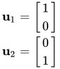
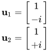
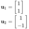
In astrophysics, an event horizon is a boundary in spacetime beyond which no signal can ever reach a given observer. Wolfgang Rindler coined the term in the 1950s.
In 1784, John Michell proposed that gravity can be strong enough in the vicinity of massive compact objects that even light cannot escape. At that time, the Newtonian theory of gravitation and the so-called corpuscular theory of light were dominant. In these theories, if the escape velocity of the gravitational influence of a massive object exceeds the speed of light, then light originating inside or from it can escape temporarily but will return. In 1958, David Finkelstein used general relativity to introduce a stricter definition of a local black hole event horizon as a boundary beyond which events of any kind cannot affect an outside observer, leading to information and firewall
paradoxes, encouraging the re-examination of the concept of local event
horizons and the notion of black holes. Several theories were
subsequently developed, some with and some without event horizons. One
of the leading developers of theories to describe black holes, Stephen Hawking, suggested that an apparent horizon
should be used instead of an event horizon, saying, "Gravitational
collapse produces apparent horizons but no event horizons." He
eventually concluded that "the absence of event horizons means that
there are no black holes – in the sense of regimes from which light
can't escape to infinity."
Any object approaching the horizon from the observer's side appears to slow down, never quite crossing the horizon. Due to gravitational redshift, its image reddens over time as the object moves closer to the horizon.
In an expanding universe, the speed of expansion reaches–and even exceeds–the speed of light, preventing signals from traveling to some regions. A cosmic event horizon is a real event horizon because it affects all kinds of signals, including gravitational waves, which travel at the speed of light.
More specific horizon types include the related but distinct absolute and apparent horizons found around a black hole. Other distinct types include:
The reachable universe as a function of time and distance, in context of the expanding Universe
In cosmology, the event horizon of the observable universe is the largest comoving distance from which light emitted now can ever reach the observer in the future. This differs from the concept of the particle horizon, which represents the largest comoving distance from which light emitted in the past
could reach the observer at a given time. For events that occur beyond
that distance, light has not had enough time to reach our location, even
if it was emitted at the time the universe began. The evolution of the
particle horizon with time depends on the nature of the expansion of the universe.
If the expansion has certain characteristics, parts of the universe
will never be observable, no matter how long the observer waits for the
light from those regions to arrive. The boundary beyond which events
cannot ever be observed is an event horizon, and it represents the
maximum extent of the particle horizon.
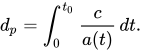
The criterion for determining whether a particle horizon for the universe exists is as follows. Define a comoving distance dp as
In this equation, a is the scale factor, c is the speed of light, and t0 is the age of the Universe. If dp→ ∞ (i.e., points arbitrarily as far away as can be observed), then no event horizon exists. If dp ≠ ∞, a horizon is present.
Examples of cosmological models without an event horizon are universes dominated by matter or by radiation. An example of a cosmological model with an event horizon is a universe dominated by the cosmological constant (a de Sitter universe).
A calculation of the speeds of the cosmological event and particle horizons was given in a paper on the FLRW cosmological model, approximating the Universe as composed of non-interacting constituents, each one being a perfect fluid.
Spacetime diagram showing a uniformly accelerated particle, P, and an event E that is outside the particle's apparent horizon. The event's forward light cone never intersects the particle's world line.
If a particle is moving at a constant velocity in a
non-expanding universe free of gravitational fields, any event that
occurs in that Universe will eventually be observable by the particle,
because the forward light cones from these events intersect the
particle's world line. On the other hand, if the particle is
accelerating, in some situations light cones from some events never
intersect the particle's world line. Under these conditions, an apparent
horizon is present in the particle's (accelerating) reference frame,
representing a boundary beyond which events are unobservable.
For example, this occurs with a uniformly accelerated particle. A spacetime diagram
of this situation is shown in the figure to the right. As the particle
accelerates, it approaches, but never reaches, the speed of light with
respect to its original reference frame. On the spacetime diagram, its
path is a hyperbola, which asymptotically approaches
a 45-degree line (the path of a light ray). An event whose light cone's
edge is this asymptote or is farther away than this asymptote can never
be observed by the accelerating particle. In the particle's reference
frame, there is a boundary behind it from which no signals can escape
(an apparent horizon). The distance to this boundary is given by , where a is the constant proper acceleration of the particle.
While approximations of this type of situation can occur in the real world (in particle accelerators,
for example), a true event horizon is never present, as this requires
the particle to be accelerated indefinitely (requiring arbitrarily large
amounts of energy and an arbitrarily large apparatus).
Interacting with a cosmic horizon
In the case of a horizon perceived by a uniformly
accelerating observer in empty space, the horizon seems to remain a
fixed distance from the observer no matter how its surroundings move.
Varying the observer's acceleration may cause the horizon to appear to
move over time or may prevent an event horizon from existing, depending
on the acceleration function chosen. The observer never touches the
horizon and never passes a location where it appeared to be.
In the case of a horizon perceived by an occupant of a de Sitter universe, the horizon always appears to be a fixed distance away for a non-accelerating observer. It is never contacted, even by an accelerating observer.
Far
away from the black hole, a particle can move in any direction, as
illustrated by the set of arrows. It is restricted only by the speed of
light.
Closer to the black hole, spacetime starts to deform. There are more paths going towards the black hole than paths moving away.
Inside
of the event horizon, all paths bring the particle closer to the centre
of the black hole. It is no longer possible for the particle to escape.
NASA
simulation (360-degree equirectangular views) of a test camera orbiting
a black hole. Due to its speed, the accretion disk appears brighter in
the direction of motion, with the black hole shadow below.
As
the camera approaches the event horizon, the view of the outside
universe appears to contract ahead while the shadow grows beneath.
Inside
of the event horizon the roles of space and time switch. The
singularity becomes an inevitable moment in the future and conversely
the event horizon becomes a moment in the past. The black hole shadow
approaches half the field of view, while simultaneously the aberration
of light (due to exponentially-increasing tidal forces) concentrate the
view of the outside universe into a thin band. In the final moments, all
views of the outside universe eventually pinch off into total darkness.
One of the best-known examples of an event horizon derives
from general relativity's description of a black hole, a celestial
object so dense that no nearby matter or radiation can escape its gravitational field. Often, this is described as the boundary within which the black hole's escape velocity is greater than the speed of light. However, a more detailed description is that within this horizon, all lightlike
paths (paths that light could take) (and hence all paths in the forward
light cones of particles within the horizon) are warped so as to fall
farther into the hole. Once a particle is inside the horizon, moving
into the hole is as inevitable as moving forward in time – no matter in
what direction the particle is travelling – and can be thought of as
equivalent to doing so, depending on the spacetime coordinate system
used.
The surface at the Schwarzschild radius acts as an event horizon in a non-rotating body that fits inside this radius (although a rotating black hole
operates slightly differently). The Schwarzschild radius of an object
is proportional to its mass. Theoretically, any amount of matter will
become a black hole if compressed into a space that fits within its
corresponding Schwarzschild radius. For the mass of the Sun, this radius is approximately 3 kilometers (1.9 miles); for Earth, it is about 9 millimeters (0.35 inches).
In practice, however, neither Earth nor the Sun have the necessary mass
(and, therefore, the necessary gravitational force) to overcome electron and neutron degeneracy pressure. The minimal mass required for a star to collapse beyond these pressures is the Tolman–Oppenheimer–Volkoff limit, which is approximately three solar masses.
According to the fundamental gravitational collapse models, an event horizon forms before the singularity of a black hole. If all
the stars in the Milky Way would gradually aggregate towards the
galactic center while keeping their proportionate distances from each
other, they will all fall within their joint Schwarzschild radius long
before they are forced to collide. Up to the collapse in the far future, observers in a galaxy surrounded
by an event horizon would proceed with their lives normally.
Black hole event horizons are widely misunderstood. Common,
although erroneous, is the notion that black holes "vacuum up" material
in their neighborhood, where in fact they are no more capable of
seeking out material to consume than any other gravitational attractor.
As with any mass in the universe, matter must come within its
gravitational scope for the possibility to exist of capture or
consolidation with any other mass. Equally common is the idea that
matter can be observed falling into a black hole. This is not possible.
Astronomers can detect only accretion disks
around black holes, where material moves with such speed that friction
creates high-energy radiation that can be detected (similarly, some
matter from these accretion disks is forced out along the axis of spin
of the black hole, creating visible jets when these streams interact
with matter such as interstellar gas or when they happen to be aimed
directly at Earth). Furthermore, a distant observer will never actually
see something reach the horizon. Instead, while approaching the hole,
the object will seem to go ever more slowly, while any light it emits
will be further and further redshifted.
The event horizon can also be defined by the causal structure of spacetime. Trajectories crossing a point in spacetime can only follow paths in a light cone
limited by the speed of light. Curvature of spacetime tips the light
cones. At the event horizon of a black hole, curvature becomes so strong
that there are no paths that lead away from the black hole.
Topologically, the event horizon is defined from the causal structure as the past null cone of future conformal timelike infinity. A black hole event horizon is teleological in nature, meaning that it is determined by future causes. More precisely, one would need to know the entire history of the
universe and all the way into the infinite future to determine the
presence of an event horizon, which is not possible for quasilocal
observers (not even in principle). In other words, there is no experiment and/or measurement that can be
performed within a finite-size region of spacetime and within a finite
time interval that answers the question of whether or not an event
horizon exists. Because of the purely theoretical nature of the event
horizon, the traveling object does not necessarily experience strange
effects and does, in fact, pass through the calculated boundary in a
finite amount of its proper time.
Interacting with black hole horizons
A misconception concerning event horizons, especially black
hole event horizons, is that they represent an immutable surface that
destroys objects that approach them. In practice, all event horizons
appear to be some distance away from any observer, and objects sent
towards an event horizon never appear to cross it from the sending
observer's point of view (as the horizon-crossing event's light cone
never intersects the observer's world line). Attempting to make an
object near the horizon remain stationary with respect to an observer
requires applying a force whose magnitude increases unboundedly
(becoming infinite) the closer it gets.
In the case of the horizon around a black hole, observers
stationary with respect to a distant object will all agree on where the
horizon is. While this seems to allow an observer lowered towards the
hole on a rope (or rod) to contact the horizon, in practice this cannot
be done. The proper distance to the horizon is finite, so the length of rope needed would be finite as well, but if the rope
were lowered slowly (so that each point on the rope was approximately at
rest in Schwarzschild coordinates), the proper acceleration (G-force)
experienced by points on the rope closer and closer to the horizon
would approach infinity, so the rope would be torn apart. If the rope is
lowered quickly (perhaps even in freefall),
then indeed the observer at the bottom of the rope can touch and even
cross the event horizon. But once this happens it is impossible to pull
the bottom of rope back out of the event horizon, since if the rope is
pulled taut, the forces along the rope increase without bound as they
approach the event horizon and at some point the rope must break.
Furthermore, the break must occur not at the event horizon, but at a
point where the second observer can observe it.
Assuming that the possible apparent horizon
is far inside the event horizon, or there is none, observers crossing a
black hole event horizon would not actually see or feel anything
special happen at that moment. In terms of visual appearance, observers
who fall into the hole perceive the eventual apparent horizon as a black
impermeable area enclosing the singularity. Other objects that had entered the horizon area along the same radial
path but at an earlier time would appear below the observer as long as
they are not entered inside the apparent horizon, and they could
exchange messages. Increasing tidal forces are also locally noticeable effects, as a function of the mass of the black hole. In realistic stellar black holes, spaghettification occurs early: tidal forces tear materials apart well before the event horizon. However, in supermassive black holes,
which are found in centers of galaxies, spaghettification occurs inside
the event horizon. A human astronaut would survive the fall through an
event horizon only in a black hole with a mass of approximately 10,000 solar masses or greater.
Beyond general relativity
A cosmic event horizon is commonly accepted as a real
event horizon, whereas the description of a local black hole event
horizon given by general relativity is found to be incomplete and
controversial. When the conditions under which local event horizons occur are modeled
using a more comprehensive picture of the way the Universe works, that
includes both relativity and quantum mechanics, local event horizons are expected to have properties that are different from those predicted using general relativity alone.
At present, it is expected by the Hawking radiation mechanism that the primary impact of quantum effects is for event horizons to possess a temperature
and so emit radiation. For black holes, this manifests as Hawking
radiation, and the larger question of how the black hole possesses a
temperature is part of the topic of black hole thermodynamics. For accelerating particles, this manifests as the Unruh effect, which causes space around the particle to appear to be filled with matter and radiation.
According to the controversial black hole firewall hypothesis, matter falling into a black hole would be burned to a crisp by a high energy "firewall" at the event horizon.
An alternative is provided by the complementarity principle,
according to which, in the chart of the far observer, infalling matter
is thermalized at the horizon and reemitted as Hawking radiation, while
in the chart of an infalling observer matter continues undisturbed
through the inner region and is destroyed at the singularity. This
hypothesis does not violate the no-cloning theorem
as there is a single copy of the information according to any given
observer. Black hole complementarity is actually suggested by the
scaling laws of strings
approaching the event horizon, suggesting that in the Schwarzschild
chart they stretch to cover the horizon and thermalize into a Planck length-thick membrane.
A complete description of local event horizons generated by gravity is expected to, at minimum, require a theory of quantum gravity. One such candidate theory is M-theory. Another such candidate theory is loop quantum gravity.
In linear algebra, an eigenvector (/ˈaɪɡən-/EYE-gən-) or characteristic vector is a (nonzero) vector that has its direction unchanged (or reversed) by a given linear transformation. More precisely, an eigenvector of a linear transformation is scaled by a constant factor when the linear transformation is applied to it: . The corresponding eigenvalue, characteristic value, or characteristic root is the multiplying factor (possibly a negative or complex number).
Geometrically, vectors are multi-dimensional quantities with magnitude and direction, often pictured as arrows. A linear transformation rotates, stretches, or shears
the vectors upon which it acts. A linear transformation's eigenvectors
are those vectors that are only stretched or shrunk, with neither
rotation nor shear. The corresponding eigenvalue is the factor by which
an eigenvector is stretched or shrunk. If the eigenvalue is negative,
then the eigenvector's direction is reversed.
The eigenvectors and eigenvalues of a linear transformation
serve to characterize it, and so they play important roles in all areas
where linear algebra is applied, from geology to quantum mechanics.
In particular, it is often the case that a system is represented by a
linear transformation whose outputs are fed as inputs to the same
transformation (feedback).
In such an application, the largest eigenvalue is of particular
importance, because it governs the long-term behavior of the system
after many applications of the linear transformation, and the associated
eigenvector is the steady state of the system.
Matrices
For an matrix and a nonzero -vector , if multiplying by (denoted ) simply scales by a factor , where is a scalar, then is called an eigenvector of , and is the corresponding eigenvalue. This relationship can be expressed as: .
Given an -dimensional vector space and a choice of basis, there is a direct correspondence between linear transformations from the vector space into itself and square matrices.
Hence, in a finite-dimensional vector space, it is equivalent to define
eigenvalues and eigenvectors using either the language of linear
transformations, or the language of matrices.
In essence, an eigenvector v of a linear transformation T is a nonzero vector that, when T is applied to it, does not change direction. Applying T to the eigenvector only scales the eigenvector by the scalar value λ, called an eigenvalue. This condition can be written as the equation
referred to as the eigenvalue equation or eigenequation. In general, λ may be any scalar. For example, λ may be negative, in which case the eigenvector reverses direction as part of the scaling, or it may be zero, or complex.
In this shear mapping,
the red arrow changes direction but the blue arrow does not. The blue
arrow is an eigenvector of this shear mapping because it does not change
direction, and since its length is unchanged, its eigenvalue is 1.A 2 × 2
real and symmetric matrix representing a stretching and shearing of the
plane. The eigenvectors of the matrix (red lines) are the two special
directions such that every point on them will just slide on them.
The example here, based on the Mona Lisa,
provides a simple illustration. Each point on the painting can be
represented as a vector pointing from the center of the painting to that
point. The linear transformation in this example is called a shear mapping.
Points in the top half are moved to the right, and points in the bottom
half are moved to the left, proportional to how far they are from the
horizontal axis that goes through the middle of the painting. The
vectors pointing to each point in the original image are therefore
tilted right or left, and made longer or shorter by the transformation.
Points along the horizontal axis do not move at all
when this transformation is applied. Therefore, any vector that points
directly to the right or left with no vertical component is an
eigenvector of this transformation, because the mapping does not change
its direction. Moreover, these eigenvectors all have an eigenvalue equal
to one, because the mapping does not change their length either.
Animated examples of eigenvectors and real eigenvalues for several non-symmetric 2D linear transformations
Linear transformations can take many different forms,
mapping vectors in a variety of vector spaces, so the eigenvectors can
also take many forms. For example, the linear transformation could be a differential operator like , in which case the eigenvectors are functions called eigenfunctions that are scaled by that differential operator, such as
Alternatively, the linear transformation could take the form of an n × n matrix, in which case the eigenvectors are n × 1 matrices.
If the linear transformation is expressed in the form of an n × n matrix A, then the eigenvalue equation for a linear transformation above can be rewritten as the matrix multiplication
where the eigenvector v is an n × 1 matrix. For a matrix, eigenvalues and eigenvectors can be used to decompose the matrix; for example, by diagonalizing it. Eigenvalues and eigenvectors give rise to many closely related mathematical concepts, and the prefix eigen- is applied liberally when naming them:
The set of all eigenvectors of a linear transformation, each paired with its corresponding eigenvalue, is called the eigensystem of that transformation.
The set of all eigenvectors of T corresponding to the same eigenvalue, together with the zero vector, is called an eigenspace, or the characteristic space of T associated with that eigenvalue.
If a set of eigenvectors of T forms a basis of the domain of T, then this basis is called an eigenbasis.
Additional animations of eigenvectors and eigenvalues in
two dimensions, including symmetric transformations and transformations
with complex eigenvalues, are available at Wikimedia Commons.
In the early 19th century, Augustin-Louis Cauchy saw how their work could be used to classify the quadric surfaces, and generalized it to arbitrary dimensions. Cauchy also coined the term racine caractéristique (characteristic root), for what is now called eigenvalue; his term survives in characteristic equation.
At the start of the 20th century, David Hilbert studied the eigenvalues of integral operators by viewing the operators as infinite matrices. He was the first to use the German word eigen, which means "own", to denote eigenvalues and eigenvectors in 1904, though he may have been following a related usage by Hermann von Helmholtz.
For some time, the standard term in English was "proper value", but the
more distinctive term "eigenvalue" is the standard today.
Eigenvalues and eigenvectors are often introduced to students in the context of linear algebra courses focused on matrices. Furthermore, linear transformations over a finite-dimensional vector space can be represented using matrices,which is especially common in numerical and computational applications.
Matrix A acts by stretching the vector x, not changing its direction, so x is an eigenvector of A.
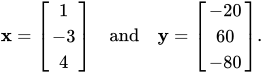
Consider two -dimensional vectors that are formed as a list of scalars, such as the three-dimensional vectors
These vectors are said to be scalar multiples of each other, or parallel, or collinear, if there is a scalar such that
In this example, .
Now consider the linear transformation of -dimensional vectors defined by an matrix :
or
where, for each row,
If it occurs that and are scalar multiples, that is, if
,
1
then is an eigenvector of the linear transformation and the scale factor is the eigenvalue corresponding to that eigenvector. Equation (1) is the eigenvalue equation for the matrix .
Equation (2) has a nonzero solution vif and only if the determinant of the matrix (A − λI) is zero. Therefore, the eigenvalues of A are values of λ that satisfy the equation
.
3
Using the Leibniz formula for determinants, the left-hand side of equation (3) is a polynomial function of the variable λ and the degree of this polynomial is n, the order of the matrix A. Its coefficients depend on the entries of A, except that its term of degree n is always (−1)nλn. This polynomial is called the characteristic polynomial of A. Equation (3) is called the characteristic equation or secular equation of A.
The characteristic polynomial of an n-by-n matrix A, being a polynomial of degree n, has at most ncomplex number
roots, which can be found by factoring the characteristic polynomial,
or numerically by root finding. The characteristic polynomial can be factored into the product of n linear terms:
,
4
where the complex numbers λ1, λ2, ..., λn,
each of which is an eigenvalue, may repeat. (The number of times an
eigenvalue appears in the characteristic polynomial is known as its algebraic multiplicity.)
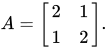
As a brief example, which is described in more detail in the examples section later, consider the matrix
Taking the determinant of (A − λI), the characteristic polynomial of A is
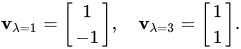
Setting the characteristic polynomial equal to zero, it has roots at λ = 1 and λ = 3, which are the two eigenvalues of A. The eigenvectors corresponding to each eigenvalue λ can be found by solving for the components of v in the equation (A − λI)v = 0. In this example, the eigenvectors are any nonzero scalar multiples of
If the entries of the matrix A
are all real numbers, then the coefficients of the characteristic
polynomial will also be real numbers, but the eigenvalues may still have
nonzero imaginary parts. The entries of the corresponding eigenvectors
therefore may also have nonzero imaginary parts. Similarly, the
eigenvalues may be irrational numbers even if all the entries of A are rational numbers or even if they are all integers. However, if the entries of A are all algebraic numbers, which include the rationals, then the eigenvalues must also be algebraic numbers.
The non-real roots of a real polynomial with real coefficients can be grouped into pairs of complex conjugates,
namely with the two members of each pair having imaginary parts that
differ only in sign and the same real part. If the degree is odd, then
by the intermediate value theorem at least one of the roots is real. Therefore, any real matrix
with odd order has at least one real eigenvalue, whereas a real matrix
with even order may not have any real eigenvalues. The eigenvectors
associated with these complex eigenvalues are also complex and also
appear in complex conjugate pairs.
Spectrum of a matrix
The spectrum
of a matrix is the list of its eigenvalues, repeated according to their
multiplicities; in a shorter notation, the set of its eigenvalues with
their multiplicities indicated.
An important quantity associated with the spectrum of a
matrix is the maximum absolute value of all of its eigenvalues. This is
known as the spectral radius of the considered matrix.
Algebraic multiplicity
Let λi be an eigenvalue of an n-by-n matrix A. The algebraic multiplicityμA(λi) of the eigenvalue is its multiplicity as a root of the characteristic polynomial, that is, the largest integer k such that (λi − λ)kevenly divides that polynomial.
Suppose a matrix A has order n and d ≤ n distinct eigenvalues. Whereas equation (4) factors the characteristic polynomial of A into the product of n linear terms with some terms potentially repeating, the characteristic polynomial can also be written as the product of d terms each corresponding to a distinct eigenvalue and raised to the power of the algebraic multiplicity:
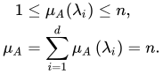
If d = n, then the right-hand side is the product of n linear terms, and this is the same as equation (4). The size of each eigenvalue's algebraic multiplicity is related to the dimension n as
If μA(λi) = 1, then λi is said to be a simple eigenvalue. If μA(λi) equals the geometric multiplicity of λi (denoted by γA(λi) and defined in the next section), then λi is said to be a semisimple eigenvalue.
Eigenspaces, geometric multiplicities, and eigenbasis for a matrix
Given a particular eigenvalue of the matrix , define the set to be all vectors that satisfy equation (2):
:\left(A-\lambda I\right)\mathbf {v} =\mathbf {0} \right\}.}
On one hand, is precisely the kernel or nullspace of the matrix . On the other hand, by definition, any nonzero vector that satisfies this condition is an eigenvector of associated with ; so is the union of the zero vector with the set of all eigenvectors of associated with . The space is called the eigenspace or characteristic space of associated with . In general, is a complex number and the eigenvectors are complex matrices (column vectors). Because every nullspace is a linear subspace of the domain, is a linear subspace of .
Because the eigenspace is a linear subspace, it is closed under addition. That is, if two vectors and belong to the set , written , then , or equivalently . This can be checked using the distributive property of matrix multiplication. Similarly, because is a linear subspace, it is closed under scalar multiplication. That is, if and , then , or equivalently . This can be checked by noting that multiplication of complex matrices by complex numbers is commutative. As long as and are not zero, they are also eigenvectors of associated with .
The dimension of the eigenspace associated with , or equivalently the maximum number of linearly independent eigenvectors associated with , is referred to as the eigenvalue's geometric multiplicity and denoted by . Because is also the nullspace of , the geometric multiplicity of is the dimension of the nullspace of , also called the nullity of . This quantity is related to the size and rank of by the equation:
Because of the definition of eigenvalues and eigenvectors, an
eigenvalue's geometric multiplicity must be at least one, that is, each
eigenvalue has at least one associated eigenvector. Furthermore, an
eigenvalue's geometric multiplicity cannot exceed its algebraic
multiplicity. Additionally, recall that an eigenvalue's algebraic
multiplicity cannot exceed . In summary,
Proof of inequality : Let B = A − λI, where λ is a fixed complex number, and the eigenspace associated with λ is the nullspace of B. Let the dimension of that eigenspace be . This means that the last k rows of the echelon form of B are zero. Thus, there is an invertible matrix E coming from Gauss-Jordan reduction, such that
Therefore the last k rows of EB − tE are (−t) times the last k rows of E. Therefore the polynomial tk evenly divides the polynomial det(EB − tE), because of basic properties of determinants (homogeneity). On the other hand, det(EB − tE) =det E det(B − tI) =pA(t + λ) det E, so (t − λ)k divides pA(t), and so the algebraic multiplicity of λ is at least . Q.E.D.
Suppose A has d ≤ n distinct eigenvalues λ1, ..., λd, where the geometric multiplicity of λi is γA(λi). The total geometric multiplicity of A,
is the dimension of the sum of all the eigenspaces of A's eigenvalues, or equivalently the maximum number of linearly independent eigenvectors of A. By construction, . If , then:
The direct sum of the eigenspaces of all of A's eigenvalues is the entire vector space .
A basis of can be formed from n linearly independent eigenvectors of A; such a basis is called an eigenbasis.
Any vector in can be written as a linear combination of eigenvectors of A.
Additional properties
Let A be an arbitrary n × n matrix of complex numbers with eigenvalues λ1, ..., λn. Each eigenvalue appears μA(λi) times in this list, where μA(λi) is the eigenvalue's algebraic multiplicity. The following are properties of this matrix and its eigenvalues:
The trace of , defined as the sum of its diagonal elements, is also the sum of all its eigenvalues:
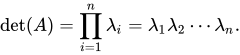
The determinant of is the product of all its eigenvalues:
For any positive integer , the eigenvalues of the th power of , that is, , are .
The eigenvalues of matrix (where is the identity matrix) are . Moreover, for any , the eigenvalues of matrix are .
More generally, for any polynomial , the eigenvalues of matrix are .
is invertible if and only if every eigenvalue is nonzero.
If is invertible, then the eigenvalues of are and for each pair of corresponding eigenvalues, the geometric multiplicities and coincide. Moreover, since the characteristic polynomial of the inverse is the reciprocal polynomial of the original up to a scalar factor, for each pair of corresponding eigenvalues, the algebraic multiplicities and coincide.
If is equal to its conjugate transpose, that is, is Hermitian, then every eigenvalue is real. The same is true of any symmetric real matrix.
If is not only Hermitian but also positive-definite, positive-semidefinite, negative-definite, or negative-semidefinite, then every eigenvalue is positive, non-negative, negative, or non-positive, respectively.
If is unitary, then every eigenvalue has absolute value .
Many disciplines traditionally represent vectors as
matrices with a single column rather than as matrices with a single row.
For that reason, the word "eigenvector" in the context of matrices
almost always refers to a 'right eigenvector', namely a column vector that right multiplies the n × n matrix A in the defining equation, equation (1),
The eigenvalue and eigenvector problem can also be defined for row vectors that left multiply matrix A. In this formulation, the defining equation is
where κ is a scalar and u is a 1 × n matrix. Any row vector u satisfying this equation is called a 'left eigenvector' of A, and κ is still called its associated eigenvalue. Taking the transpose of this equation,
Comparing this equation to equation (1), it follows immediately that a left eigenvector of is the same as the transpose of a right eigenvector of , with the same eigenvalue. Furthermore, since the characteristic polynomial of is the same as the characteristic polynomial of , the left and right eigenvectors of are associated with the same eigenvalues.
Eigenvalues of transpose
A matrix has the same eigenvalues as its transpose, as can be directly seen as follows. Assume is an eigenvalue of an matrix with eigenvector . Then ; equivalently, .
Thus, the columns of are linearly dependent. Equivalently, the rank of the matrix is less than .
But as column rank = row rank, the rows are also linearly dependent. Hence, there are numbers , not all zero, such that where the 's are the rows of . Let the row vector; then . Taking the transpose, . Moreover, is not the zero vector; so is also an eigenvalue of .
Furthermore, this argument shows that the eigenvalues of and have the same geometric multiplicity (since column nullity = row nullity).
Suppose the eigenvectors of A form a basis of , or equivalently A has n linearly independent eigenvectors v1, v2, ..., vn (with associated eigenvalues λ1, λ2, ..., λn). The eigenvectors need not be orthogonal to one another, and the eigenvalues need not be distinct. Define the square matrixQ whose columns are the n linearly independent eigenvectors of A,
Since each column of Q is an eigenvector of A, right multiplying A by Q scales each column of Q by its associated eigenvalue:
With this in mind, define the diagonal matrix Λ where each diagonal element Λii is the eigenvalue associated with the ith column of Q. Then
Because the columns of Q are linearly independent, Q is invertible. Right multiplying both sides of the equation by Q−1,
or instead left multiplying both sides by Q−1,
A
can therefore be decomposed into a matrix composed of its eigenvectors,
a diagonal matrix with its eigenvalues along the diagonal, and the
inverse of the matrix of eigenvectors. This is called the eigendecomposition; it is a similarity transformation. Such a matrix A is said to be similar to the diagonal matrix Λ, or diagonalizable. The matrix Q is the change of basis matrix of the similarity transformation. Essentially, the matrices A and Λ
represent the same linear transformation expressed in two different
bases. The eigenvectors are used as the basis when representing the
linear transformation as Λ.
Conversely, suppose a matrix A is diagonalizable. Let P be a non-singular square matrix such that P−1AP is some diagonal matrix D. Left multiplying both by P yields AP = PD. Each column of P must therefore be an eigenvector of A whose eigenvalue is the corresponding diagonal element of D. Since the columns of P must be linearly independent for P to be invertible, there exist n linearly independent eigenvectors of A.
In conclusion, the eigenvectors of form a basis of if and only if is diagonalizable.
A matrix that is not diagonalizable is said to be defective. For defective matrices, the notion of eigenvectors generalizes to generalized eigenvectors and the diagonal matrix of eigenvalues generalizes to the Jordan normal form. Over an algebraically closed field, any matrix A has a Jordan normal form and therefore admits a basis of generalized eigenvectors and a decomposition into generalized eigenspaces.
In the Hermitian case, eigenvalues can be given a variational characterization. The largest eigenvalue of H is the maximum value of the quadratic formxTHx/xTx. A value of x that realizes that maximum is an eigenvector.
Matrix examples
Two-dimensional matrix example
The transformation matrix A =⎡⎣2 11 2⎤⎦ preserves the direction of magenta vectors parallel to vλ=1 =[1 −1]T and blue vectors parallel to vλ=3 =[1 1]T.
The red vectors are not parallel to either eigenvector, so, their
directions are changed by the transformation. The lengths of the magenta
vectors are unchanged after the transformation (due to their eigenvalue
of 1), while blue vectors are three times the length of the original (due to their eigenvalue of 3). See also: An extended version, showing all four quadrants.
Consider the matrix
The figure on the right shows the effect of this transformation on point coordinates in the plane. The eigenvectors v of this transformation satisfy equation (1), and the values of λ for which the determinant of the matrix (A − λI) equals zero are the eigenvalues.
Taking the determinant to find characteristic polynomial of A,
Setting the characteristic polynomial equal to zero, it has roots at λ = 1 and λ = 3, which are the two eigenvalues of A.
For λ = 1, equation (2) becomes,
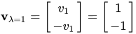
Any nonzero vector with v1 = −v2 solves this equation. Therefore,
is an eigenvector of A corresponding to λ = 1, as is any scalar multiple of this vector.
For λ = 3, equation (2) becomes
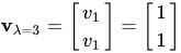
Any nonzero vector with v1 = v2 solves this equation. Therefore,
is an eigenvector of A corresponding to λ = 3, as is any scalar multiple of this vector. Thus, the vectors vλ=1 and vλ=3 are eigenvectors of A associated with the eigenvalues λ = 1 and λ = 3, respectively.
Three-dimensional matrix example
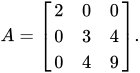
Consider the matrix
The characteristic polynomial of A is
The roots of the characteristic polynomial are 2, 1, and 11, which are the only three eigenvalues of A. These eigenvalues correspond to the eigenvectors [1 0 0]T, [0 −2 1]T, and [0 1 2]T, or any nonzero multiple thereof.
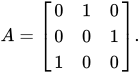
Three-dimensional matrix example with complex eigenvalues
This matrix shifts the coordinates of the vector up by one
position and moves the first coordinate to the bottom. Its
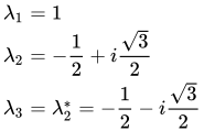
characteristic polynomial is 1 − λ3, whose roots are
where i is an imaginary unit with i2 = −1.
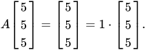
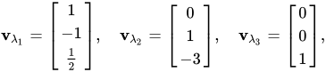
For the real eigenvalue λ1 = 1, any vector with three equal nonzero entries is an eigenvector. For example,
For the complex conjugate pair of imaginary eigenvalues,
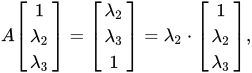
Then
and
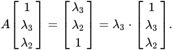
Therefore, the other two eigenvectors of A are complex and are vλ2 = [1 λ2λ3]T and vλ3 = [1 λ3λ2]T with eigenvalues λ2 and λ3, respectively. The two complex eigenvectors also appear in a complex conjugate pair,
Diagonal matrix example
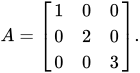
Matrices with entries only along the main diagonal are called diagonal matrices. The eigenvalues of a diagonal matrix are the diagonal elements themselves. Consider the matrix
The characteristic polynomial of A is
which has the roots λ1 = 1, λ2 = 2, and λ3 = 3. These roots are the diagonal elements as well as the eigenvalues ofA.
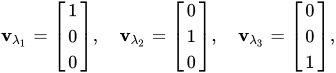
Each diagonal element corresponds to an eigenvector whose
only nonzero component is in the same row as that diagonal element. In
the example, the eigenvalues correspond to the eigenvectors,
respectively, as well as scalar multiples of these vectors.
Triangular matrix example
A matrix whose elements above the main diagonal are all zero is called a lower triangular matrix, while a matrix whose elements below the main diagonal are all zero is called an upper triangular matrix. As with diagonal matrices, the eigenvalues of triangular matrices are the elements of the main diagonal.
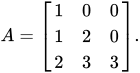
Consider the lower triangular matrix,
The characteristic polynomial of A is
which has the roots λ1 = 1, λ2 = 2, and λ3 = 3. These roots are the diagonal elements as well as the eigenvalues ofA.
These eigenvalues correspond to the eigenvectors,
respectively, as well as scalar multiples of these vectors.
Matrix with repeated eigenvalues example
As in the previous example, the lower triangular matrix
has a characteristic polynomial that is the product of its diagonal elements,
The roots of this polynomial, and hence the eigenvalues, are 2 and 3. The algebraic multiplicity
of each eigenvalue is 2; in other words they are both double roots. The
sum of the algebraic multiplicities of all distinct eigenvalues is μA =4 = n, the order of the characteristic polynomial and the dimension of A.
On the other hand, the geometric multiplicity of the eigenvalue 2 is only 1, because its eigenspace is spanned by just one vector [0 1 −1 1]T
and is therefore 1-dimensional. Similarly, the geometric multiplicity
of the eigenvalue 3 is 1 because its eigenspace is spanned by just one
vector [0 0 0 1]T. The total geometric multiplicity γA
is 2, which is the smallest it could be for a matrix with two distinct
eigenvalues. Geometric multiplicities are defined in a later section.
Eigenvector-eigenvalue identity
For a Hermitian matrixA, the norm squared of the αth
component of a normalized eigenvector can be calculated using only the
matrix eigenvalues and the eigenvalues of the corresponding minor matrix,
where is the submatrix formed by removing the αth row and column from the original matrix. This identity also extends to diagonalizable matrices. It has been discovered in and rediscovered many times in the literature.
Eigenvalues and eigenfunctions of differential operators
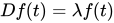
The definitions of eigenvalue and eigenvectors of a linear transformation T remains valid even if the underlying vector space is an infinite-dimensional Hilbert or Banach space. A widely used class of linear transformations acting on infinite-dimensional spaces are the differential operators on function spaces. Let D be a linear differential operator on the space of infinitely differentiable real functions of a real argument t. The eigenvalue equation for D is the differential equation
The functions that satisfy this equation are eigenvectors of D and are commonly called 'eigenfunctions'.
Derivative operator example
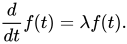
Consider the derivative operator with eigenvalue equation
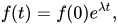
This differential equation can be solved by multiplying both sides by dt/f(t) and integrating. Its solution, the exponential function
is the eigenfunction of the derivative operator. In this case the
eigenfunction is itself a function of its associated eigenvalue. In
particular, for λ = 0 the eigenfunction f(t) is a constant.
General definition
The concept of eigenvalues and eigenvectors extends naturally to arbitrary linear transformations on arbitrary vector spaces. Let V be any vector space over some fieldK of scalars, and let T be a linear transformation mapping V into V,
We say that a nonzero vector v ∈ V is an 'eigenvector' of T if and only if there exists a scalar λ ∈ K such that
5
This equation is called the eigenvalue equation for T, and the scalar λ is the eigenvalue of T corresponding to the eigenvector v. T(v) is the result of applying the transformation T to the vector v, while λv is the product of the scalar λ with v.
Eigenspaces, geometric multiplicity, and the eigenbasis
Given an eigenvalue λ, consider the set
which is the union of the zero vector with the set of all eigenvectors associated withλ. E is called the eigenspace or characteristic space of T associated withλ. It is the kernel of the linear transformation T − λI.
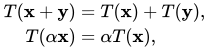
By definition of a linear transformation,
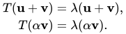
for x, y ∈ V and α ∈ K. Therefore, if u and v are eigenvectors of T associated with eigenvalue λ, namely u, v ∈ E, then
So, both u + v and αv are either zero or eigenvectors of T associated with λ, namely u + v, αv ∈ E, and E is closed under addition and scalar multiplication. The eigenspace E associated with λ is therefore a linear subspace of V. If that subspace has dimension 1, it is sometimes called an eigenline.
The geometric multiplicityγT(λ) of an eigenvalue λ is the dimension of the eigenspace associated with λ; that is, the maximum number of linearly independent eigenvectors associated with that eigenvalue. By the definition of eigenvalues and eigenvectors, γT(λ) ≥ 1 because every eigenvalue has at least one eigenvector.
The eigenspaces of T always form a direct sum. As a consequence, eigenvectors of different
eigenvalues are always linearly independent. Therefore, the sum of the
dimensions of the eigenspaces cannot exceed the dimension n of the vector space on which T operates, and there cannot be more than n distinct eigenvalues.
Any subspace spanned by eigenvectors of T is an invariant subspace of T, and the restriction of T to such a subspace is diagonalizable. Moreover, if the entire vector space V can be spanned by the eigenvectors of T, or equivalently if the direct sum of the eigenspaces associated with all the eigenvalues of T is the entire vector space V, then a basis of V called an eigenbasis can be formed from linearly independent eigenvectors of T. When T admits an eigenbasis, T is diagonalizable.
If λ is an eigenvalue of T, then the operator (T − λI) is not one-to-one, and therefore its inverse (T − λI)−1
does not exist. The converse is true for finite-dimensional vector
spaces, but not for infinite-dimensional vector spaces. In general, the
operator (T − λI) may not have an inverse even if λ is not an eigenvalue.
For this reason, in functional analysis eigenvalues can be generalized to the spectrum of a linear operatorT as the set of all scalars λ for which the operator (T − λI) has no bounded inverse. The spectrum of an operator always contains all its eigenvalues but is not limited to them.
The representation-theoretical concept of weight is an analog of eigenvalues, while weight vectors and weight spaces are the analogs of eigenvectors and eigenspaces, respectively.
The simplest difference equations have the form
The solution of this equation for x in terms of t is found by using its characteristic equation
which can be found by stacking into matrix form a set of equations consisting of the above difference equation and the k – 1 equations xt–1 = xt–1, ..., xt–k+1 = xt–k+1, giving a k-dimensional system of the first order in the stacked variable vector [xt ⋅⋅⋅xt–k+1] in terms of its once-lagged value, and taking the characteristic equation of this system's matrix. This equation gives k characteristic roots λ1, ... , λk, for use in the solution equation
The calculation of eigenvalues and eigenvectors is a topic
where theory, as presented in elementary linear algebra textbooks, is
often very far from practice.
Classical method
The classical method is to first find the eigenvalues, and
then calculate the eigenvectors for each eigenvalue. It is in several
ways poorly suited for non-exact arithmetics such as floating-point.
Eigenvalues
The eigenvalues of a matrix A can be determined by finding the roots of the characteristic polynomial. This is easy for 2 × 2 matrices, but the difficulty increases rapidly with the size of the matrix.
In theory, the coefficients of the characteristic
polynomial can be computed exactly, since they are sums of products of
matrix elements; and there are algorithms that can find all the roots of
a polynomial of arbitrary degree to any required accuracy. However, this approach is not viable in practice because the coefficients would be contaminated by unavoidable round-off errors, and the roots of a polynomial can be an extremely sensitive function of the coefficients (as exemplified by Wilkinson's polynomial). Even for matrices whose elements are integers the calculation becomes
nontrivial, because the sums are very long; the constant term is the determinant, which for an n × n matrix is a sum of n! different products.
Explicit algebraic formulas for the roots of a polynomial exist only if the degree n is 4 or less. According to the Abel–Ruffini theorem
there is no general, explicit and exact algebraic formula for the roots
of a polynomial with degree 5 or more. (Generality matters because any
polynomial with degree n is the characteristic polynomial of some companion matrix of order n.)
Therefore, for matrices of order 5 or more, the eigenvalues and
eigenvectors cannot be obtained by an explicit algebraic formula, and
must therefore be computed by approximate numerical methods. Even the exact formula for the roots of a degree 3 polynomial is numerically impractical.
Eigenvectors
Once the (exact) value of an eigenvalue is known, the
corresponding eigenvectors can be found by finding nonzero solutions of
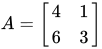
the eigenvalue equation, that becomes a system of linear equations with known coefficients. For example, once it is known that 6 is an eigenvalue of the matrix
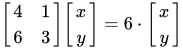
we can find its eigenvectors by solving the equation Av = 6v, that is
This matrix equation is equivalent to two linear equations
that is,
Both equations reduce to the single linear equation y = 2x. Therefore, any vector of the form [a 2a]T, for any nonzero real number a, is an eigenvector of A with eigenvalue λ = 6.
The matrix A above has another eigenvalue λ = 1. A similar calculation shows that the corresponding eigenvectors are the nonzero solutions of 3x + y = 0, that is, any vector of the form [b −3b]T, for any nonzero real number b.
The converse approach, of first seeking the eigenvectors
and then determining each eigenvalue from its eigenvector, turns out to
be far more tractable for computers. The easiest algorithm here consists
of picking an arbitrary starting vector and then repeatedly multiplying
it with the matrix (optionally normalizing the vector to keep its
elements of reasonable size); this makes the vector converge towards an
eigenvector. A variation is to instead multiply the vector by (A − μI)−1; this causes it to converge to an eigenvector of the eigenvalue closest to .
If v is (a good approximation of) an eigenvector of A, then the corresponding eigenvalue can be computed as
where v∗ denotes the conjugate transpose of v.
Modern methods
Efficient, accurate methods to compute eigenvalues and eigenvectors of arbitrary matrices were not known until the QR algorithm was designed in 1961. Combining the Householder transformation with the LU decomposition results in an algorithm with better convergence than the QR algorithm. For large Hermitiansparse matrices, the Lanczos algorithm is one example of an efficient iterative method to compute eigenvalues and eigenvectors, among several other possibilities.
Most numeric methods that compute the eigenvalues of a
matrix also determine a set of corresponding eigenvectors as a
by-product of the computation, although sometimes implementors choose to
discard the eigenvector information as soon as it is no longer needed.
Applications
Geometric transformations
Eigenvectors and eigenvalues can be useful for understanding linear transformations of geometric shapes.
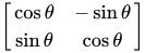
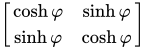
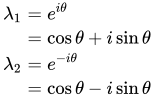
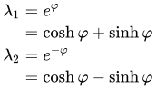
The following table presents some example transformations in the plane along with their 2 × 2 matrices, eigenvalues, and eigenvectors.
The characteristic equation for a rotation is a quadratic equation with discriminantD = −4(sin θ)2, which is a negative number whenever θ is not an integer multiple of π (180°). Therefore, except for these special cases, the two eigenvalues are complex numbers, cos θ ± isin θ;
and all eigenvectors have non-real entries. Indeed, except for those
special cases, a rotation changes the direction of every nonzero vector
in the plane.
A linear transformation that takes a square to a rectangle of the same area (a squeeze mapping) has reciprocal eigenvalues.
Principal component analysis
PCA of the multivariate Gaussian distribution centered at (1, 3) with a standard deviation of 3 in roughly the (0.878, 0.478) direction and of1 in the orthogonal direction. The vectors shown are unit eigenvectors of the (symmetric, positive-semidefinite) covariance matrix
scaled by the square root of the corresponding eigenvalue. Just as in
the one-dimensional case, the square root is taken because the standard deviation is more readily visualized than the variance.
In spectral graph theory, an eigenvalue of a graph is defined as an eigenvalue of the graph's adjacency matrixA, or (increasingly) of the graph's Laplacian matrix due to its discrete Laplace operator, which is either D − A (sometimes called the combinatorial Laplacian) or I − D−1/2AD−1/2 (sometimes called the normalized Laplacian), where D is a diagonal matrix with Dii equal to the degree of vertex vi, and in D−1/2, the ith diagonal entry is . The kth principal eigenvector of a graph is defined as either the eigenvector corresponding to the kth largest or kth
smallest eigenvalue of the Laplacian. The first principal eigenvector
of the graph is also referred to merely as the principal eigenvector.
The principal eigenvector is used to measure the centrality of its vertices. An example is Google's PageRank algorithm. The principal eigenvector of a modified adjacency matrix of the World Wide Web graph gives the page ranks as its components. This vector corresponds to the stationary distribution of the Markov chain
represented by the row-normalized adjacency matrix; however, the
adjacency matrix must first be modified to ensure a stationary
distribution exists. The second smallest eigenvector can be used to
partition the graph into clusters, via spectral clustering. Other methods are also available for clustering.
Markov chains
A Markov chain is represented by a matrix whose entries are the transition probabilities
between states of a system. In particular the entries are non-negative,
and every row of the matrix sums to one, being the sum of probabilities
of transitions from one state to some other state of the system. The Perron–Frobenius theorem
gives sufficient conditions for a Markov chain to have a unique
dominant eigenvalue, which governs the convergence of the system to a
steady state.
Vibration analysis
Mode shape of a tuning fork at eigenfrequency 440.09Hz
Eigenvalue problems occur naturally in the vibration analysis of mechanical structures with many degrees of freedom. The eigenvalues are the natural frequencies (or 'eigenfrequencies')
of vibration, and the eigenvectors are the shapes of these vibrational
modes. In particular, undamped vibration is governed by
or
That is, acceleration is proportional to position (i.e., we expect x to be sinusoidal in time).
The orthogonality properties of the eigenvectors allows decoupling of the differential equations
so that the system can be represented as linear summation of the
eigenvectors. The eigenvalue problem of complex structures is often
solved using finite element analysis, but neatly generalize the solution to scalar-valued vibration problems.
In solid mechanics, the stress tensor is symmetric and so can be decomposed into a diagonal
tensor with the eigenvalues on the diagonal and eigenvectors as a
basis. Because it is diagonal, in this orientation, the stress tensor
has no shear components; the components it does have are the principal components.
An example of an eigenvalue equation where the transformation T is represented in terms of a differential operator is the time-independent Schrödinger equation in quantum mechanics:
where the HamiltonianH is a second-order differential operator, and the wavefunctionψE is one of its eigenfunctions corresponding to the eigenvalue E, interpreted as its energy.
However, in the case where one is interested only in the bound state solutions of the Schrödinger equation, one looks for ψE within the space of square integrable functions. Since this space is a Hilbert space with a well-defined scalar product, one can introduce a basis set in which ψE and H
can be represented as a one-dimensional array (i.e., a vector) and a
matrix respectively. This allows one to represent the Schrödinger
equation in a matrix form.
The bra–ket notation
is often used in this context. A vector, which represents a state of
the system, in the Hilbert space of square integrable functions is
represented by |ΨE⟩. In this notation, the Schrödinger equation is:
where |ΨE⟩ is an 'eigenstate' of H, and E represents the eigenvalue. H is an observableself-adjoint operator, the infinite-dimensional analog of Hermitian matrices. As in the matrix case, in the equation above H|ΨE⟩ is understood to be the vector obtained by application of the transformation H to |ΨE⟩.
Wave transport
Light, acoustic waves, and microwaves are randomly scattered numerous times when traversing a static disordered system.
Even though multiple scattering repeatedly randomizes the waves,
ultimately coherent wave transport through the system is a deterministic
process which can be described by a field transmission matrix t. The eigenvectors of the transmission operator t†t
form a set of disorder-specific input wavefronts which enable waves to
couple into the disordered system's eigenchannels: the independent
pathways waves can travel through the system. The eigenvalues, τ, of t†t
correspond to the intensity transmittance associated with each
eigenchannel. One of the remarkable properties of the transmission
operator of diffusive systems is their bimodal eigenvalue distribution
with τmax = 1 and τmin = 0. Furthermore, one of the striking properties of open eigenchannels,
beyond the perfect transmittance, is the statistically robust spatial
profile of the eigenchannels.
In geology, especially in the study of glacial till,
(roughly the rock below the ice), eigenvectors and eigenvalues are used
to represent data about orientation. When the data is given in the form
eigenvalue, eigenvector
azimuth◦, eigenvector
plunge◦, this allows understanding the eigenvector's orientation in a
real world setting. The three different eigenvalues of the three eigenvectors describing a
sample can be compared to determine a possible preferred direction of
orientation.
The basic reproduction number (R0)
is a fundamental number in the study of how infectious diseases spread.
If one infectious person is put into a population of completely
susceptible people, then R0
is the average number of people that one typical infectious person will
infect. The generation time of an infection is the time, tG,
from one person becoming infected to the next person becoming infected.
In a heterogeneous population, the next generation matrix defines how
many people in the population will become infected after time tG has passed. The value R0 is then the largest eigenvalue of the next generation matrix.
In image processing, processed images of faces can be seen as vectors whose components are the brightnesses of each pixel. The dimension of this vector space is the number of pixels. The eigenvectors of the covariance matrix associated with a large set of normalized pictures of faces are called eigenfaces; this is an example of principal component analysis. They are very useful for synthesizing images as a linear combination of vectors. In the facial recognition branch of biometrics, eigenfaces provide a means of applying data compression to faces for identification purposes. Research related to eigen vision systems determining hand gestures has also been made.
Similar to this concept, eigenvoices
represent the general direction of variability in human pronunciations
of a particular utterance, such as a word in a language. Based on a
linear combination of such eigenvoices, a new voice pronunciation of the
word can be constructed. These concepts have been found useful in
automatic speech recognition systems for speaker adaptation.




.jpg)
.jpg)
.jpg)









































![{\displaystyle {\begin{aligned}\det(A-\lambda I)&=\left|{\begin{bmatrix}2&1\\1&2\end{bmatrix}}-\lambda {\begin{bmatrix}1&0\\0&1\end{bmatrix}}\right|={\begin{vmatrix}2-\lambda &1\\1&2-\lambda \end{vmatrix}}\\[6pt]&=3-4\lambda +\lambda ^{2}\\[6pt]&=(\lambda -3)(\lambda -1).\end{aligned}}}](https://wikimedia.org/api/rest_v1/media/math/render/svg/852afe30ae1c99b2f2ff91b62e226d28cef2609a)


![{\displaystyle {\begin{aligned}\det(A-\lambda I)&=\left|{\begin{bmatrix}2&0&0\\0&3&4\\0&4&9\end{bmatrix}}-\lambda {\begin{bmatrix}1&0&0\\0&1&0\\0&0&1\end{bmatrix}}\right|={\begin{vmatrix}2-\lambda &0&0\\0&3-\lambda &4\\0&4&9-\lambda \end{vmatrix}},\\[6pt]&=(2-\lambda ){\bigl [}(3-\lambda )(9-\lambda )-16{\bigr ]}=-\lambda ^{3}+14\lambda ^{2}-35\lambda +22.\end{aligned}}}](https://wikimedia.org/api/rest_v1/media/math/render/svg/bdfec3c58ac4306d8cc19110ac4b2b5bfbea234e)